Lihua Li* | Yazhou Xing | Peng Wen | Yao Yu | Congcong Li | Renlu Huang
OPEN ACCESS
The rectal temperature is traditionally measured and taken as the body temperature of chickens. However, there is not yet a correlation model between body temperature and rectal temperature to reflect the dynamic change law of chicken body temperature in real time. To solve the problem, this paper establishes a correlation model between the wing temperature and rectal temperature of chickens based on genetic programming (GP). Then, the competitive selection method was applied to optimize the data on wing temperature and rectal temperature of chickens under room temperature. The competitive size was set to 5, and the optimization was terminated when the individual fitness remained unchanged in 3 consecutive generations. The model was run independently 40 times, and verified with the data on wing temperature and rectal temperature of chickens under cold stress. The results show that the mean absolute value of error was 0.025 for the fitting between wing and rectal temperatures, and the prediction error of the model was 0.17 %. Therefore, our model can automatically search for optimal relation function of rectal temperature and wing temperature and achieve a high fitting accuracy. The research provides a novel and rapid temperature measurement method for chickens.
monitoring devices, layer, wing temperature, GP, data-simulation, body temperature monitoring
The change of body temperature can reflect the health condition of chickens. The body temperature of diseased chicken could reach 43~44 °C. To discover the diseases in time, it is necessary to detect the body temperature and observe the change curve of body temperature [1, 2]. During the diagnosis of chicken diseases, the rectal temperature is traditionally measured and taken as the body temperature. The measurement usually lasts 3~5min. This approach has a poor real-time performance, causes a huge stress on chickens, and exposes operators to infection sources. If there are many chickens, it is time-consuming and inefficient to measure the rectal temperature one by one. Then, the operators cannot discover the diseased individuals in time, putting the entire flock in danger. This calls for accurate, real-time detection of the body temperature of chickens.
With the technical advancement of wireless sensors, many monitoring devices have been developed to measure the body temperature of poultry. For example, Winget et al. [3] used the implanted telemetry system to draw the change curve of body temperature of roosters and hens under continuous illumination. Cain and Wowilson [4] monitored the circadian rhythm, activities and laying temperature of chickens with a multi-channel telemetry system. Okada et al. [5-8] developed a wearable wireless sensor monitoring system, and applied it to simulate the bird flu in a chicken farm. The simulation results show that, if 5 % of all chicken wear sensors, the bird flue could be detected 2 days earlier than manual monitoring; the wireless sensors are small and light, but fail to satisfy the requirement on power consumption of data transmission. Li [9] designed a real-time monitoring device of wing temperature of chickens. In the device, the node design full considers the needs of chicken. However, the nodes are powered by large batteries with a short life, making the device difficult to wear for a long term.
With the aid of genetic programming (GP), this paper establishes a correlation model between the wing temperature and rectal temperature of chickens, providing a new method to measure the body temperature of chickens easily and safely. The research offers a new way to prevent, control and prewarn chicken diseases.
2.1 GP introduction
Genetic programming (GP), established by Professor. Koza of Stanford University, is one new branch of evolutionary computation. The GP is valid in terms of symbolic regression, displaying strong problem-solving ability. The symbolic regression, also called as function modelling, means to find the fitting function relation according to one set of given independent variable and function values. In the GP algorithm design, five tasks should be pre-defined, including terminal set T, initial function set F, evaluation method of fitness value, operation control quantity and the termination standard, where the genetic manipulation, evaluation of fitness value and initial genetic programming are the key [10, 11].
Refer to the detailed steps as follows.
Step 1: Determine the objective function. Given the input and output samples as X={(x11, x12, …, x1m), (x21, x22, …, x2m)(xn1, xn2, …, xnm)}, Y= {y1,y2, …, yn}. The programming design is aimed to determine one best function expression. And the G (c, x1, x2, …, xm) can minimize the error: minf=|∑G(c, xk1, xk2, …, xkm)-yk| (k=1, 2, …,n) Where c is real constant.
Step 2: Make encoding. Determine terminal set T and function set F; define the elements of T as variable x and constant c.
Step 3: Initialize the parent generation group. Given the group size as N, then N trees are generated altogether. Take the minimum integer for the maximum depth (number of layers) of these trees, to make explanation for the best function expression searched by GP. At the generation of N trees as the initial group, the root node of every tree can be randomly selected in the corresponding coded values of the function set F, the intermediate nodes in the corresponding coded values of the union set D, and the leaf nodes in the corresponding values of terminal set T.
Step 4: Make decoding of parent generation group and fitness evaluation.
Step 5: Make genetic, crossover and mutation operation for parent generation group.
Step 6: Take records of the best individual, and choose the offspring as the new parent generation group. Then repeat the steps from step 4, until the iterations of evolution are over the pre-defined value, or the objective function reaches the pre-defined value. The best obtained now is the final result [12-13].
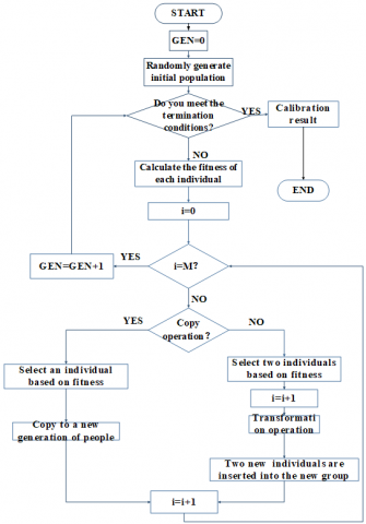
2.2 GP algorithm flow
Figure 1. Genetic programming algorithm flow
Refer to the GP algorithm in the following:
(1) Determine the operator set and data set of the model;
(2) Initialize the population of tree expression. Generate n populations of initial tree expressions at random;
(3) Repeat the steps above, until meeting all termination conditions;
1) Evaluate each individual in the population, and make fitness computation for every individual.
2) Based on the crossover probability and fitness value, randomly select the individual to take the following two steps and then generate the new-generation individual;
a) Duplicate the existing individual to the new population;
b) Generate one new individual by hybridization of the two individuals.
(4) The best individual may appear in any generation, as the final result by the genetic programming.
Figure 1 depicts the flow chart of genetic programming algorithm, where M is number of individuals in the population, i is the index number of individuals in the population, and GEN is the current algebra [14-16].
3.1 Data collection
In this test, select 40 healthy hy-line variety grey layer at about 40-week old with less individual difference and more similar weight 1.415±0.162Kg. Make artificial heating and humidification of the temperature in the test chicken house, and monitor the real-time environment to reach the internal temperature 20±2 ⁰C and relative humidity 70±4 %. Then take measurements of wing temperature and rectal temperature in 30-minute cycle: the former is to measure the temperature of hairless area under the wing; the latter is to measure the rectal temperature in the cloacae. To collect the wing temperature and rectal temperature in the violent changes of environmental temperatures, the test group and control group were made respectively in the test. For each group, firstly, pre-treat them for 12h in the enclosed indoor environment, and then start the test simultaneously. In 10h cold stress, transfer the test group to the enclosed house for 4h, and measure the wing temperature and rectal temperature every 30 minutes. Make real-time synchronous monitoring of the outdoor environment by the monitoring equipment.
3.2 Data processing
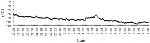
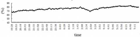
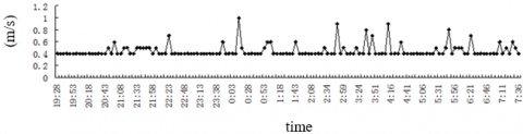
Outdoor environment changes and indoor environment
(1) Average temperature in outdoor environment: -8.68±2.12 ⁰C; average relative humidity: 76.05±18.59 %; average wind velocity: 0.42±0.01 m/s. The changes are shown in the following:
Figure 2. Changes of outdoor temperature
Figure 3. Change of outdoor relative humidity
Figure 4. Change of outdoor wind velocity
(2) Indoor environment: average temperature: 21±2 ⁰C; average relative humidity: 75±4 %; average wind velocity less than 0.4m/s.
3.3 Change rule of chicken body temperature in the test condition
In the test, process the data in Excel 2003, use SPSS (13.0) statistics software for variance analysis, and compare the data with the mean value ± standard deviation ( ±SD).
Table 1 shows, in the cold stress outdoors, the wing temperature and rectal temperature of the test group decreased respectively: in the cold stress process (19:30-05:30), the rectal temperature of the test group was lower than in control group, while in the recovery process indoors (5:30-9:30), it was higher than in control group; in the cold stress process (19:30-05:30), the wing temperature in test group was lower than in control group, while in the recovery process (5:30-9:30), it was higher than in control group.
Table 1. Variation of rectal temperature and under-wing temperature during the experiment
|
Time |
RT (⁰C) |
RC (⁰C) |
WT (⁰C) |
WC (⁰C) |
RT-RC (⁰C) |
WT-WC (⁰C) |
|
19:30 |
40.80 ±0.17 |
40.93 ±0.06 |
40.22 ±0.30 |
40.35 ±0.40 |
-0.13 ±0.12 |
-0.09 ±0.38 |
|
20:00 |
40.80 ±0.10 |
41.03 ±0.15 |
40.04 ±0.30 |
40.10 ±0.62 |
-0.23 ±0.21 |
-0.01 ±0.56 |
|
20:30 |
40.77 ±0.06 |
41.00 ±0.30 |
40.42 ±0.56 |
40.48 ±0.73 |
-0.23 ±0.31 |
-0.02 ±1.04 |
|
21:00 |
40.70 ±0.00 |
41.07 ±0.25 |
40.38 ±0.45 |
40.80 ±0.76 |
-0.37 ±0.25 |
-0.39 ±1.00 |
|
21:30 |
40.80 ±0.10 |
41.23 ±0.06 |
40.28 ±0.48 |
41.05 ±0.54 |
-0.43 ±0.06 |
-0.74 ±0.94 |
|
22:00 |
40.63 ±0.06 |
41.07 ±0.06 |
39.80 ±0.60 |
40.85 ±0.76 |
-0.43 ±0.06 |
-0.99 ±1.15 |
|
22:30 |
40.43 ±0.06 |
40.97 ±0.15 |
39.26 ±1.30 |
40.28 ±0.78 |
-0.53 ±0.15 |
-1.08 ±1.44 |
|
23:00 |
40.37 ±0.15 |
40.93 ±0.15 |
39.22 ±0.86 |
40.63 ±0.52 |
-0.57 ±0.15 |
-1.41 ±1.25 |
|
23:30 |
40.33 ±0.21 |
40.97 ±0.15 |
39.22 ±0.54 |
40.43 ±0.87 |
-0.63 ±0.12 |
-1.25 ±0.45 |
|
0:00 |
40.30 ±0.10 |
41.00 ±0.35 |
39.46 ±0.72 |
40.75 ±0.53 |
-0.70 ±0.26 |
-1.29 ±0.97 |
|
0:30 |
40.37 ±0.15 |
41.07 ±0.25 |
39.82 ±0.61 |
40.53 ±0.57 |
-0.70 ±0.17 |
-0.70 ±0.90 |
|
1:00 |
40.23 ±0.15 |
40.90 ±0.26 |
39.64 ±0.59 |
40.20 ±0.68 |
-0.67 ±0.31 |
-0.55 ±1.04 |
|
1:30 |
40.23 ±0.06 |
40.83 ±0.12 |
39.00 ±0.65 |
40.05 ±0.60 |
-0.60 ±0.10 |
-1.04 ±1.09 |
|
2:00 |
40.33 ±0.06 |
40.77 ±0.06 |
40.02 ±0.44 |
40.00 ±0.78 |
-0.43 ±0.12 |
0.03 ±1.08 |
|
2:30 |
40.37 ±0.12 |
40.80 ±0.00 |
39.18 ±0.86 |
40.28 ±0.82 |
-0.43 ±0.12 |
-1.09 ±1.03 |
|
3:00 |
40.33 ±0.15 |
40.83 ±0.12 |
38.36 ±1.57 |
40.00 ±0.78 |
-0.50 ±0.26 |
-1.59 ±2.09 |
|
3:30 |
40.33 ±0.23 |
40.67 ±0.06 |
39.42 ±0.44 |
39.63 ±0.55 |
-0.33 ±0.29 |
-0.18 ±0.90 |
|
4:00 |
40.33 ±0.15 |
40.83 ±0.06 |
39.50 ±0.78 |
39.43 ±0.81 |
-0.50 ±0.20 |
0.08 ±1.27 |
|
4:30 |
40.30 ±0.00 |
40.93 ±0.06 |
38.86 ±0.96 |
39.33 ±0.79 |
-0.63 ±0.06 |
-0.47 ±1.44 |
|
5:00 |
40.33 ±0.12 |
40.80 ±0.10 |
39.24 ±0.65 |
39.33 ±0.79 |
-0.47 ±0.15 |
-0.09 ±1.06 |
|
5:30 |
40.43 ±0.06 |
40.80 ±0.00 |
39.00 ±0.58 |
39.75 ±0.64 |
-0.37 ±0.06 |
-0.72 ±0.83 |
|
6:00 |
40.70 ±0.10 |
40.67 ±0.06 |
39.92 ±0.37 |
39.45 ±0.66 |
0.03 ±0.15 |
0.46 ±0.72 |
|
6:30 |
40.90 ±0.26 |
40.80 ±0.10 |
40.16 ±0.91 |
39.65 ±0.58 |
0.10 ±0.20 |
0.54 ±1.28 |
|
7:00 |
40.83 ±0.25 |
40.67 ±0.12 |
39.92 ±0.87 |
39.10 ±0.54 |
0.17 ±0.15 |
0.84 ±1.25 |
|
7:30 |
40.87 ±0.29 |
40.60 ±0.17 |
40.44 ±0.47 |
39.05 ±0.48 |
0.27 ±0.12 |
1.41 ±0.81 |
|
8:00 |
40.83 ±0.25 |
40.73 ±0.15 |
40.20 ±0.41 |
39.50 ±0.51 |
0.10 ±0.10 |
0.65 ±0.55 |
|
8:30 |
40.97 ±0.12 |
40.80 ±0.10 |
40.44 ±0.42 |
39.68 ±0.57 |
0.17 ±0.06 |
0.80 ±0.54 |
|
9:00 |
40.87 ±0.06 |
40.93 ±0.12 |
40.34 ±0.32 |
39.70 ±0.61 |
-0.07 ±0.15 |
0.67 ±0.39 |
|
9:30 |
40.80 ±0.10 |
41.07 ±0.23 |
40.28 ±0.38 |
40.01 ±0.80 |
-0.27 ±0.32 |
0.27±0.39 |
Note: RT and RC stand for the test group and control group for rectal temperature respectively; WT and WC the test group and control group for wing temperature respectively; RT-RC and WT-WC mean the test group -the control group for rectal temperature, and the test group-control group for wing temperature respectively.
Figure 5. Change curve of layer wing temperature and rectal temperature in the test
Refer to Figure 5 for the change curve of layer wing temperature and rectal temperature in the test.
3.4 GP-based model construction of layer temperature
3.4.1 Parameter setting
The parameters in genetic programming algorithm greatly depends on the computation accuracy and operation speed. In this paper, given the terminal set as T={x, R1, R2, R3} and function set as F={+, -, *, /, sqrt, sin, cos, exp, ln}. Apply the competitive selection method, with the competitive size as 5. Stop the optimization if population evolution for G generations or no change of the fitness values for the best individual in the three generations continuously; then make independent operation for 40 times. The other parameters are shown in Table 2.
Table 2. GP model parameter
|
Control parameters |
Value |
|
Max. algebra |
1000 |
|
Max. scale |
500 |
|
Duplication probability |
0.2 |
|
Exchange probability |
0.9 |
|
Mutation probability |
0.05 |
|
Max. tree of initial individual |
5 |
|
Generation method for initial group |
Ramped half-and-half creation method |
|
Termination criterion |
Specified max. permissible algebra |
Fitting result of wing temperature and rectal temperature relation
By the measured data in Table 1, this paper applies the genetic programming to find the regression function and then obtains the relation function of rectal temperature and wing temperature:
YGP=(X1+(((sin(X1))+(Exp(((sin(R3))*((Exp(((sin((sin(X1))))+(Exp(((sin((sin(X1))))*(Exp((Exp((Log(R1))))))))))))*((sin((R2+((sin(X1))+(R2+(sin(X1)))))))+R1))))))+(Exp(((sin(((Log((R2+(sin(R2)))))+X1)))*(Log(((((R2*(sin((R3+R3))))+(sin(((((Log(R2))+(((sin(X1))+(Exp(((sin(R3))*R2))))+(Exp(R1))))+(((sin(((Log(R3))-(Exp(X1)))))+R2)+((Exp(X1))+(((R2+R3)+(Exp(R3)))*R2))))+(Exp(((sin((Exp(((sin(R2))+(X1+R1))))))*R3)))))))+(sin(((((((Log(((sin(R1))+R2)))+((((sin(R3))*(Log(R2)))+R1)+(Exp(R1))))+(((sin((X1-R2)))+R1)+((Exp(X1))+(((R2+R3)+(Exp(R3)))*R2))))+(Exp(((sin(((R2+(sin(R2)))+((X1*X1)*(R3+X1)))))*(Log(X1))))))+(sin((Exp((((sin((X1*X1)))+((Log(X1))+(Log(R2))))+R2))))))+(Exp(((sin(((Log((R2+R1)))+(Exp(((sin((X1*X1)))+(R2+(Log(R2)))))))))*(Log(X1)))))))))+(sin((((sin((((Log(((R2+((R2+R2)+(sin(R2))))+(sin(((R2+X1)+(R3*X1)))))))-(sin((R3*X1))))/(R2*(sin(((sin(X1))+(Exp(((sin(R3))*(X1+R3)))))))))))+(sin((((sin((((Log((Log(X1))))-(sin((R3*X1))))/(R2*(sin((sin(R1))))))))+(sin((Exp((sin((Exp((sin(R3)))))))))))+(Exp(((sin((X1+(Exp((R3+R2))))))*(Log(X1)))))))))+(Exp(((sin(((Log(R2))+(Exp(((sin(((sin(X1))*(Exp(R3)))))+(R2+(sin((Exp(R2)))))))))))*(Log(X1))))))))))))))));
where, X1-measured value of wing temperature (⁰C); YGP-fitting value of rectal temperature (⁰C”; R1=0.60595; R2=7.17509; R3=3.80456.
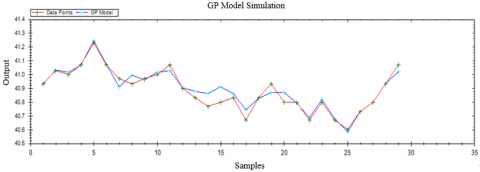
Refer to fitting data in Table 3, and the fitting chart in Figure 6, with the mean absolute value of error 0.025.
Figure 6. Fitting chart of genetic programming
Table 3. Fitting data of wing temperature and rectal temperature relation
|
Wing temperature (⁰C) |
Rectal temperature (⁰C) |
GP Design (⁰C) |
GP absolute error |
|
40.35 |
40.93 |
40.93 |
0 |
|
40.1 |
41.03 |
41.03 |
0 |
|
40.48 |
41 |
41.01 |
0.01 |
|
40.8 |
41.07 |
41.07 |
0 |
|
41.05 |
41.23 |
41.24 |
0.01 |
|
40.85 |
41.07 |
41.07 |
0 |
|
40.28 |
40.97 |
40.91 |
0.06 |
|
40.63 |
40.93 |
40.99 |
0.06 |
|
40.43 |
40.97 |
40.96 |
0.01 |
|
40.75 |
41 |
41.01 |
0.01 |
|
40.53 |
41.07 |
41.03 |
0.04 |
|
40.2 |
40.9 |
40.9 |
0 |
|
40.05 |
40.83 |
40.87 |
0.04 |
|
40 |
40.77 |
40.85 |
0.08 |
|
40.28 |
40.8 |
40.91 |
0.11 |
|
40 |
40.83 |
40.85 |
0.02 |
|
39.63 |
40.67 |
40.74 |
0.07 |
|
39.43 |
40.83 |
40.83 |
0 |
|
39.33 |
40.93 |
40.87 |
0.06 |
|
39.33 |
40.8 |
40.86 |
0.06 |
|
39.75 |
40.8 |
40.79 |
0.01 |
|
39.45 |
40.67 |
40.68 |
0.01 |
|
39.65 |
40.8 |
40.81 |
0.01 |
|
39.1 |
40.67 |
40.67 |
0 |
|
39.05 |
40.6 |
40.58 |
0.02 |
|
39.5 |
40.73 |
40.73 |
0 |
|
39.68 |
40.8 |
40.79 |
0.01 |
|
39.7 |
40.93 |
40.93 |
0 |
|
40.01 |
41.07 |
41.02 |
0.05 |
|
Mean absolute error 0.025 |
|||
3.5 Model application and result analysis
Table 4. Fitting data of wing temperature and rectal temperature in cold stress
|
Rectal temperature (⁰C) |
Wing temperature (⁰C) |
GP design (⁰C) |
GP absolute error |
|
40.22 |
40.8 |
40.79 |
0.01 |
|
40.42 |
40.77 |
40.772 |
0.002 |
|
40.38 |
40.7 |
40.72 |
0.02 |
|
40.28 |
40.8 |
40.81 |
0.01 |
|
39.8 |
40.63 |
40.62 |
0.01 |
|
39.26 |
40.43 |
40.43 |
0 |
|
39.22 |
40.37 |
40.37 |
0 |
|
39.22 |
40.33 |
40.36 |
0.03 |
|
39.46 |
40.3 |
40.32 |
0.02 |
|
39.82 |
40.37 |
40.4 |
0.03 |
|
39.64 |
40.23 |
40.29 |
0.06 |
|
39 |
40.23 |
40.34 |
0.11 |
|
40.02 |
40.33 |
40.36 |
0.03 |
|
39.18 |
40.37 |
40.33 |
0.04 |
|
38.36 |
40.33 |
40.32 |
0.01 |
|
39.42 |
40.33 |
40.31 |
0.02 |
|
39.5 |
40.33 |
40.33 |
0 |
|
38.86 |
40.3 |
40.3 |
0 |
|
39.24 |
40.33 |
40.31 |
0.02 |
|
39 |
40.43 |
40.34 |
0.09 |
|
39.92 |
40.7 |
40.73 |
0.03 |
|
40.16 |
40.9 |
40.9 |
0 |
|
39.92 |
40.83 |
40.8 |
0.03 |
|
40.44 |
40.87 |
40.91 |
0.04 |
|
40.2 |
40.83 |
40.8 |
0.03 |
|
40.44 |
40.97 |
40.8 |
0.17 |
|
40.34 |
40.87 |
40.87 |
0 |
|
40.28 |
40.8 |
40.81 |
0.01 |
|
Mean absolute error 0.029 |
|||
The model is verified by the rectal temperature and wing temperature data of the test group in Table 1; the results are shown in Table 4, with the mean absolute value of error 0.029, meeting the real-time monitoring demands of layer production temperature.
To compare the GP model and the traditional prediction methods, the stepwise regression model and backpropagation neural network (BPNN) were both adopted to predict the rectal temperature of chickens. From the data measured under cold stress, some data not used for modelling were taken as the test samples, and imported into the GP, BPNN and stepwise regression model. The prediction results are given in Tables 5 and 6.
Table 5. Prediction results of the three models
|
Measured results |
GP results |
BPNN results |
Stepwise regression results |
|
40.8 |
40.72 |
40.6 |
40.4 |
|
40.77 |
40.7 |
40.63 |
40.53 |
|
40.7 |
40.75 |
40.58 |
40.54 |
|
40.8 |
40.86 |
40.73 |
40.66 |
|
40.63 |
40.52 |
40.6 |
40.43 |
|
40.43 |
40.34 |
40.1 |
40.07 |
|
40.37 |
40.3 |
40.21 |
40.42 |
|
40.33 |
40.26 |
40.23 |
40.5 |
|
39.46 |
39.4 |
39.21 |
39.17 |
|
39.82 |
39.78 |
39.61 |
39.54 |
|
No. |
GP error % |
BPNN error % |
Stepwise regression error % |
|
1 |
-0.20 |
-0.49 |
-0.98 |
|
2 |
-0.17 |
-0.34 |
-0.59 |
|
3 |
0.12 |
-0.29 |
-0.39 |
|
4 |
0.15 |
-0.17 |
-0.34 |
|
5 |
-0.27 |
-0.42 |
-0.49 |
|
6 |
-0.22 |
-0.82 |
-0.89 |
|
7 |
-0.17 |
-0.40 |
0.12 |
|
8 |
-0.17 |
-0.25 |
0.42 |
|
9 |
-0.15 |
-0.63 |
-0.73 |
|
10 |
-0.10 |
-0.53 |
-0.70 |
|
Total |
0.17 |
0.43 |
0.46 |
Based on the BP, this paper designs a model for the relationship between rectal temperature and wing temperature of chickens. In this model, the functional relationship is searched for automatically by the BP, and fitted automatically at a high accuracy.
Using the data measured under cold stress, the GP model was compared with the BPNN and the stepwise regression model. The results show that the BP model predicted the rectal temperature more accuracy than the contrastive models. Through evolutionary computation, this model can automatically look for the best function about the relationship between rectal temperature and wing temperature of chickens. The research findings provide a new and effective method for chicken production and a valuable reference for chicken disease diagnosis.
This paper was supported by National Key R&D Program of China (2018YFD0800100); research and development of intelligent equipment and information technology for livestock and poultry breeding (2018YFD0500700); the two-stage innovation team of modern agricultural industry technology system in Hebei (HBCT2018150208); Hebei Excellent Program for Overseas Students Introduction (CN201704).
[1] Lacey, B., Hamrita, T.K., Lacy, M.P., Van Wicklen, G.L. (2000). Assessment of poultry deep body temperature responses to ambient temperature and relative humidity using an online telemetry system. Transactions of the ASAE, 43(3): 717-721. https://doi.org/10.13031/2013.2754
[2] Deeb, N., Cahaner, A. (2001). The effects of high ambient temperature on dwarf versus normal broilers. Poultry Science, 80(5): 541-548. https://doi.org/10.1093/ps/80.6.695
[3] Winget, C.M., Averkin, E.G., Fryer, T.B. (1965). Quantitative measurement by telemetry of ovulation and oviposition in the fowl. American Journal of Physiology, 209(4): 853-858. https://doi.org/10.1152/ajplegacy.1965.209.4.853
[4] Cain, J.R., Wilson, W.O. (1971). Multichannel telemetry system for measuring body temperature: circadian rhythms of body temperature, locomotor activity and oviposition in chickens. Poultry Science, 50(5): 1437-1443. https://doi.org/10.3382/ps.0501437
[5] Okada, H., Itoh, T., Suzuki, K., Tsukamoto, K. (2009). Wireless sensor system for detection of avian influenza outbreak farms at an early stage. Sensors, 1374-1377. https://doi.org/10.1109/ICSENS.2009.5398422
[6] Okada, H., Itoh, T., Suzuki, K., Tatsuya, T., Tsukamoto, K. (2010). View All Authors Simulation study on the wireless sensor-based monitoring system for rapid identification of avian influenza outbreaks at chicken farms. Sensors,660-663. https://doi.org/10.1109/ICSENS.2010.5690089
[7] Okada, H., Nogami, H., Itoh, T., Masuda, T. (2012). Development of low power technologies for health monitoring system using wireless sensor nodes. The Workshop on Design, 90-95. https://doi.org/10.1109/dMEMS.2012.13
[8] Okada, H., Nogami, H., Kobayashi, T., Masuda, T., Itoh, T. (2013). Development of ultra-low power wireless sensor node with piezoelectric accelerometer for health monitoring. 2013 Transducers & Eurosensors XXVII: The 17th International Conference on Solid-State Sensors, Actuators and Microsystems (Transducers & Euro sensors XXVII), pp. 26-29. https://doi.org/10.1109/Transducers.2013.6626692
[9] Li, L.H., Huang, R.L., Huo, L.M., Li, J.X., Chen, H. (2012). Design and experiment on monitoring device for layers individual production performance parameters. Transactions of the Chinese Society of Agricultural Engineering, 28(4): 160-164. https://doi.org/10.3969/j.issn.1002-6819.2012.04.026
[10] Liu, D.Y., Lu, Y.N., Wang, F. (2001). Genetic programming paradigm: A survey. Journal of Computer Research and Development, 38(2): 213-222.
[11] Chen, X.N., Jia, Q., Han, L.M., Guo, F., Liu, G. (2009). Application of genetic programming for calibration of flowmeter in the middle route of south-to-north water transfer project. South-to-North Water Transfers and Water Science & Technology, 6(7): 290-293. https://doi.org/10.3969/j.issn.1672-1683.2009.06.076
[12] Liu, Y., Su, X.Y. (2010). Genetic programming theory and it's application. Microcomputer Information, 9(26): 115-117. https://doi.org/10.3969/j.issn.2095-6835.2010.27.046
[13] Hirasawa, K., Okubo, M., Katagiri, H., Hu, J., Murata, J. (2001). Comparison between genetic network programming (GNP) and genetic programming (GP). Proceedings of the IEEE Conference on Evolutionary Computation, ICEC, 2: 1276-1282. https://doi.org/10.1109/CEC.2001.934337
[14] Koza, J.R., Bennett, F.H., Keane, M.A., Andre, D. (1997). Automatic programming of a time-optimal robot controller and an analog electrical circuit to implement the robot controller by means of genetic programming. Proceedings of IEEE International Symposium on Computational Intelligence in Robotics and Automation, 340-346. https://doi.org/10.1109/CIRA.1997.613878
[15] Keijzer, M., Baptist, M.J., Babovic, V., Uthurburu, J.R. (2005). Determining equations for vegetation induced resistance using genetic programming. Proceeding GECCO '05 Proceedings of the 7th annual conference on Genetic and evolutionary computation, pp. 1999-2006. https://doi.org/10.1145/1068009.1068343
[16] Azamathulla, H.M.D., Ghani, A.A.B., Zakaria, N.A., Lai, S.H., Chang, C.K., Leow, C.S., Abuhasan, Z. (2008). Genetic programming to predict ski-jump bucket spill way scour. Journal of Hydrodynamics, 20(4): 477-484. https://doi.org/10.1016/s1001-6058(08)60083-9