Haddouche Mohammed Reda* | Benazza Abdelylah
OPEN ACCESS
The biggest problem that can be encountered in the Parabolic Trough Collector is the tube wear, and this is due to the non-uniformity of the temperature distribution over the circumferential angle of the tube. In this paper the absorber tube is moved downward away the focal line of the parabola and a secondary reflector is added overhead the tube in order to reduce the heat flux gradient and homogenize it. The simulation method of the ray’s path is adopted by Soltrace software. The numerical results of the enhanced Parabolic Trough Collector show that the heat flux gradient can be enhanced and reduced by 70.37 % and the temperature gradient can be reduced from 159.39 K to 24.16 K by adding the secondary reflector.
heat transfer enhancement, parabolic trough collector, non-uniform heat flux, Nusselt number, secondary reflector, computational fluid dynamic
The absorber tube is the major component and the key parameter of a parabolic trough solar collector. The non-uniformity of the solar flux distribution over the outer surface of the absorber tube leads to a large difference on the temperature distribution which can cause damages and failures. Nowadays the researchers and engineers in the field search to decrease the circumferential temperature gradient to avoid failures and increase the life time of the absorber tube.
Moreover, many researchers focus on the heat transfer enhancement between the absorber tube and the heat transfer fluid using different methods. Jie Deng et al. [1] investigated the heat transfer enhancement of a receiver tube by introducing concentric and eccentric rod inserts and using molten salt as HTF. Their results show that the usage of rod insert can enhance the heat transfer performance and reduces of the maximum tube wall temperature. Gong Xiangtao et al. [2] analysed the Heat transfer enhancement of a parabolic trough solar receiver with pin-fin arrays inserting. Their results show that the use of pin-fin arrays inserting increases the overall heat transfer performance and decreases the temperature gradient of the absorber tube. Xingwang Song et al. [3] carried out a numerical study of parabolic trough receiver with non-uniform heat flux and helical screw-tape inserts. They investigated the effect of solar incidence angle on heat flux distribution, the heat loss of a receiver, the maximum temperature on absorber tube outer surface and the maximum circumferential temperature difference. Some researchers tried to modify the shape and the geometry of the parabolic trough collector. Bin Zou et al. [4] presented a detailed study on the optical performance of parabolic trough solar collectors with Monte Carlo Ray Tracing method. Their results prove that the geometrical parameters, including aperture width, focal length and absorber diameter, have great effects on the optical performance of the PTC and the distribution of local concentration ratio around the absorber tube varies greatly with different geometrical configurations and for some special parameter conditions. Yassine Demagh et al. [5, 6] analysed the feasibility of an S-curved sinusoidal absorber of parabolic trough collector using Tonatiuh code to establish the heat flux density on the outer surface of the absorbers. Their results show that the highest values of the heat flux density decrease, what leads to reduce the temperature gradient; they concluded also that the S-curved absorber should be comparatively better than the conventional straight absorber tube. Tao Tao et al. [7] analysed a new trough solar concentrator. Their analysis shows that the trough width of the system is the important factor that determines the performance of the system. Fei Cao et al. [8, 9] analysed the thermal performance and stress of the elliptical cavity receiver tube in the parabolic trough solar collector. Panna Lal Singh et al. [10] studied experimentally the heat loss of trapezoidal cavity absorbers for linear solar concentrating collector. Their results show that the values of the heat loss coefficient for the trapezoidal cavity absorber were lower as compared to the concentric glass covered absorber. X. Xiao et al. [11] analysed experimentally and numerically the heat transfer of a V-cavity absorber for linear parabolic trough solar collector. They found that the V-cavity absorber with the rectangular fins has a better heat transfer performance. And the average outlet temperature of the heat transfer fluid increases and the temperature of the heating surface decreases adding rectangular fins, which confirms that the rectangular fins in the absorber can enhance the heat transfer and decrease the heat loss. A. Kajavali et al. [12] investigated the heat transfer enhancement in a parabolic trough collector with a modified absorber. Their numerical analysis conducted that the single tube absorber showed a lower solar energy recovery than the modified absorber. Wang Kun et al. [13] presented a numerical study for a new type parabolic trough solar collector with uniform solar flux distribution. Their analysis show that the solar flux distribution can be homogenized by adding a secondary reflector which leads to reduce significantly the maximum temperature and the circumferential temperature difference of the absorber tube wall.
In this paper the absorber tube is moved downward away the focal line and a secondary parabola is added to reduce the heat flux gradient over the circumferential angle of the absorber tube and increase the reliability of the absorber tube.
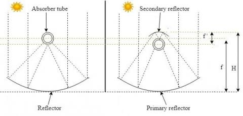
The conventional parabolic trough collector is designed to capture the direct solar irradiance over a large parabolic shaped surface and concentrate it onto its focal line. The concentrator is a sheet metal bended to a parabolic shape and painted with reflective surface to reflect solar irradiation on its focal line. The absorber tube is the major component of PTC, in which solar radiation is focused and converted to thermal energy by an intermediate of a heat transfer fluid (HTF). From (Figure 1a) it can be seen that the absorber tube is subjected to a non-uniform heat flux while the bottom periphery of is subjected to concentrated solar radiation and the top one is subjected to non-concentrated solar radiation. The non-uniformity of the solar flux distribution over the outer surface of the absorber tube leads to a large difference on the temperature distribution which can cause damages.
In order to homogenize the heat flux and reduce the circumferential temperature gradient; the absorber tube is moved away from the focal line of the parabolic trough concentrator toward the concentrator and a secondary reflector is added overhead the tube. The two parabolas are arranged in an opposite manner. The sun rays reflected by the primary concentrator hit the bottom part of the absorber tube and a portion of these rays are reflected again on the upper part of the absorber tube by the secondary reflector as shown in (Figure 1b). Table 1 shows the geometrical parameters of the Parabolic Trough Collector.
Figure 1. The schematic diagram of the parabolic trough collector
Table 1. The geometrical parameters of the parabolic trough collector
|
Focal length of the primary concentrator (f) Focal length of the secondary reflector (f’) Distance of the secondary reflector (H) Aperture width of the primary concentrator Aperture width of the secondary concentrator Absorber tube inner radius Absorber tube outer radius Transmittance of the glass pipe Cover inner radius Cover outer radius |
1.71 m 0.011m 1.76 m 5.77 m 0.09 m 3.2 cm 3.5 cm 96 % 5.95 cm 6.25 cm |
3.1 The MCRT simulation
The simulation of the Local Concentration Ration (LCR) of the conventional PTC and PTC with secondary reflector is adopted by SolTrace software developed at the National Renewable Energy Laboratory (NREL) to model concentrating solar power optical systems and analyse their performance and it is based on the Monte Carlo Ray Tracing method (MCRT).
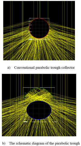
Figure 2 shows the path of the rays reflected by the concentrator on the absorber tube. It can be seen from this figure that the absorber tube of the conventional PTC (Figure 2a) is subjected to a concentrated solar flux on the bottom part while the upper one is subjected to a non-concentrated solar flux; and by moving the absorber tube downward and adding a secondary reflector; the solar rays can reach the upper part after reflected by the additional reflector as shown in Figure 2b.
Figure 2. Ray’s path reflected by the concentrator on the absorber tube
3.2 The CFD simulation
3.2.1 Governing equations
The equations which govern the computational fluid dynamics are continuity, momentum, energy and the standard k-ɛ equations [1]:
Continuity equation
$\frac{\partial }{\partial {{x}_{j}}}\left( \rho {{u}_{i}} \right)=0$ (1)
Momentum equation
$\frac{\partial }{\partial {{x}_{i}}}\left( \rho {{u}_{i}}{{u}_{j}} \right)=-\frac{\partial P}{\partial {{x}_{i}}}+\frac{\partial }{\partial {{x}_{j}}}\left[ \begin{align} & \left( \mu +{{\mu }_{t}} \right)\left( \frac{\partial {{u}_{i}}}{\partial {{x}_{j}}}+\frac{\partial {{u}_{j}}}{\partial {{x}_{i}}} \right) \\ & -\frac{2}{3}\left( \mu +{{\mu }_{t}} \right)\frac{\partial {{u}_{i}}}{\partial {{x}_{i}}}{{\delta }_{ij}} \\\end{align} \right]+\rho {{g}_{i}}$ (2)
Energy equation
$\frac{\partial }{\partial {{x}_{i}}}\left( \rho {{u}_{i}}T \right)=\frac{\partial }{\partial {{x}_{i}}}\left[ \left( \frac{\mu }{\Pr }+\frac{{{\mu }_{t}}}{{{\sigma }_{t}}} \right)\frac{\partial T}{\partial {{x}_{i}}} \right]$ (3)
The standard k-ɛ model has two model equations, one for k and one for ɛ [14]:
k-equation
$\begin{align} & \frac{\partial }{\partial {{x}_{i}}}\left( \rho {{u}_{i}}k \right)=\frac{\partial }{\partial {{x}_{i}}}\left[ \left( \mu +\frac{{{\mu }_{t}}}{{{\sigma }_{k}}} \right)\frac{\partial k}{\partial {{x}_{i}}} \right] \\ & +{{G}_{k}}-\rho \varepsilon \\\end{align}$ (4)
ɛ- equation
$\begin{align} & \frac{\partial }{\partial {{x}_{i}}}\left( \rho {{u}_{i}}\varepsilon \right)=\frac{\partial }{\partial {{x}_{i}}}\left[ \left( \mu +\frac{{{\mu }_{t}}}{{{\sigma }_{\varepsilon }}} \right)\frac{\partial \varepsilon }{\partial {{x}_{i}}} \right] +\frac{\varepsilon }{k}\left( {{c}_{1\varepsilon }}{{G}_{k}}-{{c}_{2\varepsilon }}\rho \varepsilon \right) \\\end{align}$ (5)
where, Gk represent the generation of turbulent kinetic energy
${{G}_{k}}={{\mu }_{t}}\frac{\partial {{u}_{i}}}{\partial {{x}_{i}}}\left( \frac{\partial {{u}_{i}}}{\partial {{x}_{j}}}+\frac{\partial {{u}_{j}}}{\partial {{x}_{i}}} \right)+\frac{2}{3}\rho k{{\delta }_{ij}}\frac{\partial {{u}_{i}}}{\partial {{x}_{j}}}$ (6)
In these equations, turbulent viscosity µtis defined as:
${{\mu }_{t}}={{c}_{\mu }}\rho \frac{{{k}^{2}}}{\varepsilon }$ (7)
The equations contain five adjustable constants Cµ, σk, σɛ, c1ɛ and c2ɛ. This model employs values for the constants that are arrived at by comprehensive data fitting for a wide range of turbulent flow [15]:
Cµ=0.09, σk =1.00 σɛ=1.30 c1ɛ=1.44 and c2ɛ=1.92.
3.2.2 Boundary conditions
$Q=LCR\cdot DNI$ (8)
where, the DNI is the Direct normal irradiance (DNI=1000 W/m2).
${{T}_{sky}}=0.00552\cdot T_{amb}^{1.5}$ (9)
where, Tamb is ambient temperature (Tamb=300 K)
And the convective heat transfer coefficient of the wind is given by [18]:
$hw=4V_{w}^{0.58}\cdot d_{go}^{-0.48}$ (10)
where, Vw is the wind speed, (Vw=2.5 m/s) and dgo is the glass cover outer diameter.
The HTF used in this study is the Therminol®VP1. It is a eutectic mixture of 73.5 % diphenyl oxide and 26.5 % diphenyl and as such can be used in existing liquid or vapor systems.
All the equations are discretised by the finite volume method. All the equations are solved by the first order scheme, the coupling between the pressure and the velocity is based on the simple algorithm [15]. The thermo-physical properties of the fluid are taken constant.
For this purpose the numerical results are compared with correlations obtained from literature. The average Nusselt Number is given by:
$\overline{Nu}=\frac{h{{d}_{ai}}}{\lambda }$ (11)
And
$\overline{h}=\frac{\overline{Q}}{{{T}_{ai}}-{{T}_{f}}}$ (12)
where, Q is the average heat flux on the absorber tube, Tai is the average temperature of the inner wall of the absorber tube and Tf is the average temperature of the HTF.
The Darcy friction factor for turbulent flow is defined as:
$f=\frac{2{{d}_{ai}}\Delta P}{L\rho {{u}^{2}}}$ (13)
where, dai and L are the inner diameter and the length of the absorber tube respectively.
The Nusselt number given by Gnielinski [18] is defined as:
$Nu=\frac{\frac{f}{8}\left( \operatorname{Re}-1000 \right)\Pr }{1+12.7{{\left( \frac{f}{8} \right)}^{0.5}}\left( {{\Pr }^{\frac{2}{3}}}-1 \right)}$ (14)
where, the friction factor f can be determined from an appropriate relation such as the first Petukhov’s equation [18, 19] for turbulent flow in smooth tube:
$f={{\left( 0.79\ln \operatorname{Re}-1.64 \right)}^{-2}}$ (15)
For 0.5 ≤Pr≤2000 and 3000≤Re≤5x10^6
Another equation presented by Notter [18] to determine the average Nusselt number:
$Nu=5+0.015{{\operatorname{Re}}^{0.856}}{{\Pr }^{0.347}}$ (16)
Blasius [17] proposed a correlation to calculate the Darcy friction factor for fully developed flow inside circular smooth tubes:
$f=0.184{{\operatorname{Re}}^{-0.2}}$ (17)
For Re > 2x10^4
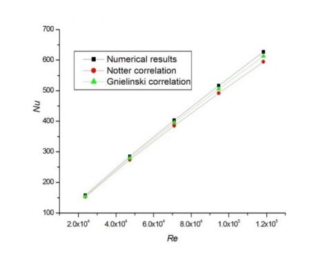
Figure 3 and Figure 4 show the comparison between the numerical results and the results calculated by correlations obtained from literature of the Nusselt number Nu and the Darcy friction factor f respectively. From these figures, it can be seen that the curves agree well with each other with a maximum deviation of 2.14 % for Nu number and the maximum error for the friction factor is 2.78 %.
Figure 3. Variation of Nu number as a function of Re number
Figure 4. Variation of f number as a function of Re number
5.1 Ray tracing and heat flux analysis
In the first part of this this paper; the LCR obtained from Soltrace software for both the conventional PTC and the PTC with secondary reflector are investigated.
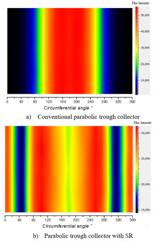
Figure 5 shows the flux map of the conventional PTC and the enhanced PTC. From these figures it can be seen that the heat flux of the conventional PTC is non-uniform with a large gradient while by adding a secondary reflector the gradient of the flux decreases and becomes homogenous.
Figure 5. Flux map of the conventional PTC and the enhanced PTC
Figure 6. Variation of f number as a function of Re number
The LCR for both conventional PTC and the PTC with secondary reflector are shown in (Figure 6) .It can be seen that the LCR decreases and becomes slightly uniform by adding the secondary reflector and the maximum value of the heat flux decreases to 31000 W/m² and the minimum value increases to 15000 W/m², while for the conventional PTC the peak value is 55000 W/m² and the minimum value is 1000 W/m². The gradient of the heat flux over the circumferential angle of the absorber tube is enhanced and reduced by 70.37 %.
5.2 Temperature distribution analysis
In the second part of this study; the thermal performance and the efficiency of the conventional PTC and the PTC with the secondary reflector are investigated under the same conditions.
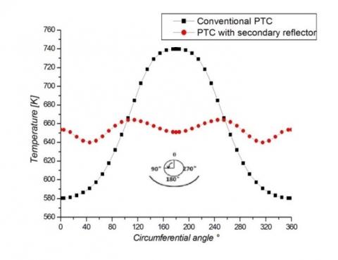
Figure 7 presents the temperature distribution over the circumferential angle of both the conventional PTC and the enhanced one at the middle distance L=2m and for Re=47.31x10^4. It can be seen that the temperature gradient is reduced significantly and becomes homogenous. It can be also noticed that by adding a secondary reflector the maximum temperature is decreased from 739.84 K to 663.98 K and the minimum temperature is increased from 580.44 K to 639.82 K, and the temperature gradient difference is reduced from 159.39 K to 24.16 K.
Figure 7. The temperature distribution on the outer surface of the absorber tube as a function of circumferential angle
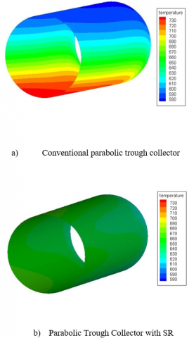
Figure 8. The contour of the temperature distribution of the absorber tube
The contour of temperature distribution over the wall of both conventional tube and tube with secondary reflector are shown in Figure 6. From this figure it can be seen that that the temperature distribution of the conventional PTC (Figure 8a) is non-uniform and by adding another reflector the temperature distribution becomes more uniform (Figure 8b)
In this paper the heat flux distribution on the outer surface of the absorber tube of Parabolic Trough Collector is investigated and enhanced in order to reduce the temperature gradient of the tube by moving the absorber tube away from the focal line toward the parabola and adding a secondary reflector. The numerical results of the soltrace software indicate that the heat flux distribution is enhanced and the heat flux gradient can be reduced by adding another reflector overhead the absorber tube by 70.37 %, also the numerical results of the computational Fluid Dynamics show that the maximum temperature is decreased from 739.84 K to 663.98 K and the minimum temperature is increased from 580.44 K to 639.82 K, and the temperature gradient difference is reduced from 159.39 K to 24.16 K.
|
CP |
specific heat, J. kg-1. K-1 |
|||
|
f L |
Friction factor Receiver length, |
|||
|
Nu P Pr Q Re T V |
Nusselt number Pressure, Pa Prandtl number Heat flux, W.m-2.K-1 Reynolds number Temperature, K Velocity, m.s-1 |
|||
|
Greek symbols
|
|
|
||
|
ɛ |
emissivity |
|
||
|
λ |
Thermal conductivity, W.m-2. K-1 |
|
||
|
ρ |
solid volume fraction |
|
||
|
µ |
dynamic viscosity, kg. m-1.s-1 |
|
||
|
|
|
|
||
|
Subscripts
|
|
|
||
|
a |
Absorber |
|
||
|
e |
Envelope |
|
||
|
i o f sky w a |
Inner Outer fluid Sky Wall Ambience |
|
||
[1] Chang, C, Sciacovelli, A., Wu, Z.Y., Li, X., Li, Y.L., Zhao, M.Z., Deng, J., Wang, Z.F., Ding, Y.L. (2018). Enhanced heat transfer in a parabolic trough solar receiver by inserting rods and using molten salt as heat transfer fluid. Applied Energy, 220: 337-350. https://doi.org/10.1016/j.apenergy.2018.03.091
[2] Bejan, A. (2015). Constructal thermodynamics. International Journal of Heat and Technology, 34(Special Issue 1): S1-S8. https://doi.org/10.18280/ijht.34S101
[3] Gong, X.T., Wang, F.Q., Wang, H.Y., Tan, J.Y., Lai Q.Z., Han, H.Z. (2017). Heat transfer enhancement analysis of tube receiver for parabolic trough solar collector with pin fin arrays inserting. Solar Energy, 144: 185-202. https://doi.org/10.1016/j.solener.2017.01.020
[4] Song, X.W., Dong, G.B., Gao, F.Y., Diao, X.G., Zheng, L.Q., Zhou, F.Y. (2014). A numerical study of parabolic trough receiver with nonuniform heat flux and helical screw-tape inserts. Energy, 77: 771-782. https://doi.org/10.1016/j.energy.2014.09.049
[5] Zou, B., Dong, J.K., Yao, Y., Jiang, Y.Q. (2017). A detailed study on the optical performance of parabolic trough solar collectors with Monte Carlo Ray Tracing method based on theoretical analysis. Solar Energy, 147: 189-201. https://doi.org/10.1016/j.solener.2017.01.055
[6] Demagh, Y., Bordja, I., Kabar, Y., Benmoussa, H. (2015). A design method of an S-curved parabolic trough collector absorber with a three-dimensional heat flux density distribution. Solar Energy, 122: 873-884. https://doi.org/10.1016/j.solener.2015.10.002
[7] Demagh, Y. (2018). Numerical investigation of a novel sinusoidal tube receiver for parabolic trough technology. Applied Energy, 218: 494-510. https://doi.org/10.1016/j.apenergy.2018.02.177
[8] Tao, T., Zheng, H.F., He, K.Y., Abdulkarim, M. (2011). A new trough solar concentrator and its performance analysis. Solar Energy, 85: 198-207. https://doi.org/10.1016/j.solener.2010.08.017
[9] Cao, F., Wang, L., Zhu, T.Y. (2017). Design and optimization of elliptical cavity tube receivers in the parabolic trough solar collector. International Journal of Photoenergy, 2017: 7 pages. https://doi.org/10.1155/2017/1471594
[10] Singh, P.L., Sarviya, R.M., Bhagoria, J.L. (2010). Heat loss study of trapezoidal cavity absorbers for linear solar concentrating collector. Energy Conversion and Management, 51(2): 329-337. https://doi.org/10.1016/j.enconman.2009.09.029
[11] Xiao, X., Zhang, P., Shao, D.D., Li, M. (2014). Experimental and numerical heat transfer analysis of a V-cavity absorber for linear parabolic trough solar collector. Energy Conversion and Management, 86: 49-59. https://doi.org/10.1016/j.enconman.2014.05.001
[12] Kajavali, A., Sivaraman, B., Kulasekharan, N. (2014). Investigation of heat transfer enhancement in a parabolic trough collector with a modified absorber. International Energy Journal, 14(4): 177-188.
[13] Wang, K., He, Y.L., Cheng, Z.D. (2014). A design method and numerical study for a new type parabolic trough solar collector with uniform solar flux distribution. Science China Technological Sciences, 57(3): 531-540. https://doi.org/10.1007/s11431-013-5452-6
[14] Launder, B.E., Splanding, D.B. (1974). The numerical computation of turbulent flows. Computer Methods in Applied Mechanics ANR Engineering, 3(2): 269-289. https://doi.org/10.1016/0045-7825(74)90029-2
[15] Versteeg, H.K., Malalasekera, W. (1995). An introduction to computational fluid dynamics. The Finite Volume Method. John Wiley and Sons Ink, New York.
[16] Swinbank, W.C. (1963). Long-wave radiation from clear skies. Quarterly Journal of the Royal Meteotological Society, 89(31): 339-348. https://doi.org/10.1002/qj.49708938105
[17] Mullick, S.C., Nanda, S.K. (1989). An improved technique for computing the heat loss factor of a tubular absorber. Solar Energy, 42(1): 1-7. https://doi.org/10.1016/0038-092X(89)90124-2
[18] Yunus, A.C. (2007). Heat and Mass Transfer: A Practical Approach. (Third eds), MC Graw Hill.
[19] Petukhov, B.S. (1970). Heat transfer and friction in turbulent pipe flow with variable physical properties. Advances in Heat Transfer, 6: 504-561. https://doi.org/10.1016/S0065-2717(08)70153-9
[20] Notter, R.H., Sleicher, C.A. (1972). A solution to the turbulent Graetz problem-III Fully developed and entry region heat transfer rates. Chemical Engineering Science, 27: 2073-2093.