Fethi Albouchi* | Foued Mzali | Salah Saadaoui | Abdelmajid Jemni
OPEN ACCESS
In this paper an electro-thermal method is used for measuring the thermal conductivity of liquids. This technique is based on eight heat sensing resistors which are connected to form a Wheatstone bridge. Measurements performed on several liquids covering a wide range of thermal properties validate the method. The total standard uncertainty of the experimental results was estimated to be less than 3.8 %. Good agreement is found between the measured values of the thermal properties and previously reported values in literature. Moreover, measurements using this method are less time consuming than using the classical methods. This technique may find practical application for the thermal characterization of complex fluids even when applying external electric or magnetic fields.
thermal conductivity, liquids, electro-thermal method, Wheatstone bridge, Hot bridge
Thermal conductivity of heat transfer fluids plays a vital role in the development of high performance heat-exchange devices. In energy applications such as automobile engine and electronic chips, basic fluids like water and ethylene glycol are used for cooling. For these cooling fluids, the thermal conductivity is a very important property which is taken into account in designing and controlling the process.
Generally, measurements of the thermophysical properties of liquids are quite difficult and present some problems. These problems are related to the coupling of conduction with convective and radiative heat transfers.
A comprehensive review of the main methods used for the measurement of the thermal conductivity of fluids is given in [1]. These measured methods can be classified into two types [2]. The first one, named the steady-state techniques, are well developed, but are expensive in equipment and are practically difficult in operation. The second type is named the unsteady-state methods which can be divided in two kinds electrothermal and photothermal techniques. Only few works deal with the use of photothermal methods for characterization of liquids. Schriempf was the first to develop an apparatus dedicated to measurement on liquids [3]. The inconvenient of its method is that it is not adaptable for low thermal conductivity. Farooq et al. [4] proposed a similar approach based on a three-layered cell using an original sample holder made of outside layers brazed to a ring-shaped central spacer. Remy and Degiovanni [5-6] show that liquids present some difficulties since several mode of heat transfer are coupled. In their works, a theoretical study and an experimental approach based on the flash method are developed in order to determine the thermal parameters of liquids.
The Flash method is also adapted by Coquard and Panel [7] for the thermal characterization of liquids and pasty materials. They give a new technique for the computation of the thermal conductivity based on a 3-D simulation of the transient heat transfer in the axisymmetric composite sample.
Among, the unsteady electrothermal methods, the transient hot wire (THW) becomes one of commonly used techniques for the measurement of the thermal conductivity of liquids [8, 17]. In its standard configuration, a thin metal wire introduced in a liquid sample, acts as a resistive heat source and a thermometer. The voltage drop across the wire provides a measure of the thermal conductivity. For this method, to have a significant value of resistance, the hot wire should have a very thin diameter, which is sometimes difficult experimentally.
All the mentioned techniques present some inconvenient even in the experimental set-up or in the theoretical formulation. The intension of this paper is to overcame these problems and to present a method with quick experimental runs. This technique has a robust design suitable for many industrial applications, giving that it doesn’t require specific fluid enclosure and have easy experimental procedure. This method is based on the transient hot-bridge (THB) [18-20], which has previously shown its efficiency with the classical identification procedure based on slop calculation for determining thermal conductivity of solids. In this paper, the THB is adapted to liquids with a new identification procedure, based on the instantaneous slope versus time. It is based on a thermoelectrical sensor composed of four strips; each one is segmented into two parts of different lengths and connected to form a Wheatstone bridge. The bridge is inherently balanced. A constant current is passed through the bridge to heat the resistances, thus resulting in unbalancing of the bridge due to the resistance change.
Different liquid is characterized by this method. The thermal conductivity is measured with a good accuracy. These obtained results are compared with literature values and a good agreement is obtained.
This procedure could find applications for the measurements of numerous materials such as biological tissues or food materials for which other classical measuring methods are not suitable.
The remainder of this paper is organized as follows: Section 1 introduces the theoretical formulation. Section 2 describes the experimental set-up and the measurement process. In the section 3, we present the obtained results and we finish with a conclusion.
2.1 Analytical model
The sensor is constituted of four parallel tandem strips. Each tandem strip comes in two individual striplets, a short and a long one. Two of the tandems are placed very close to each other at the centre of the sensor and one tandem on either edge (Figure 1).
Figure 1. Top view of the sensor
The eight striplets are symmetrically switched for an equal-resistance Wheatstone bridge. The electrical circuit is represented on Figure 2.
Figure 2. Equivalent circuit diagram of the sensor
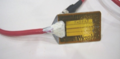
Figure 3. Sensor
The sensor is mounted on an aluminum plate so that the Wheatstone bridge can be in direct contact with the fluid (Figure 3). As long as the sample temperature is uniform, the bridge is inherently balanced. An electric current flowing through the resistances turns the bridge into an unbalanced condition. The high-sensitivity output-signal of the sensor is practically not affected by ambient electrical noise and allows measuring the thermal conductivity of the surrounding medium.
The thermal conductivity is calculated from the slope of the output-signal UB versus time in a logarithmic scale, ln(t) . Another identification method, using the instantaneous slope mi and time ti values allows for sufficiently precise determination of the thermal conductivity.
In this case, the voltage drop of a long segment is reduced to that of a short. The output signal UB of the sensor with supply current IB is formed only from the middle segments of the four strips. So, the difference of the temperature rises between inner and outer strips is defined by:
$\text{ }\!\!\Delta\!\!\text{ }T={{T}_{\text{inn}}}-{{T}_{\text{out}}}$ (1)
where the temperature rises on the inner and outer strips are the sum of the temperatures rises seen from the strips themselves and from other strips with distance Di. In this case, we can write:
${{T}_{\text{inn}}}=T\left( {{D}_{0}} \right)+T\left( {{D}_{1}} \right)+T\left( {{D}_{3}} \right)+T\left( {{D}_{4}} \right)$ (2)
and
${{T}_{\text{out}}}=T\left( {{D}_{0}} \right)+T\left( {{D}_{2}} \right)+T\left( {{D}_{3}} \right)+T\left( {{D}_{4}} \right)$ (3)
Replacing Eqns (2, 3) in the equation (1), we obtain:
$\Delta T=T({{D}_{1}})-T({{D}_{2}})$ (4)
The temperature rise from a hot strip is given by [19]:
$T\left( t \right)-{{T}_{0}}=\frac{-q}{4\pi \lambda }\cdot Ei\left( -\frac{{{D}^{2}}}{4at} \right)$ (5)
where D is the strip width and Ei is the exponential integral.
Substituting the Eq. (5) into Eq. (4), we obtain the basic equation of the sensor method:
$\Delta T\left( t \right)=\frac{q}{4\pi \lambda }\left[ Ei\left( -\frac{D_{2}^{2}}{4at} \right)-Ei\left( -\frac{D_{1}^{2}}{4at} \right) \right]$ (6)
The conductivity identification is based on the calculation of the output signal slope, which can be written as [19]:
$\frac{d\left( \Delta T\left( t \right) \right)}{d\left( Ln\left( t \right) \right)}=\frac{q}{4\pi \lambda }\left[ -\exp \left( -\frac{D_{2}^{2}}{4at} \right)+\exp \left( -\frac{D_{1}^{2}}{4at} \right) \right]=\frac{q}{4\pi \lambda }\times m\left( t \right)$ (7)
with m(t)=mi is the adimentioned instantaneous slope.
Based on Eq. (7), the maximum slope is obtained for t=tmax, so one can write:
$\frac{d\left( \Delta T\left( {{t}_{\max }} \right) \right)}{d\left( Ln\left( {{t}_{\max }} \right) \right)}=\frac{q}{4\pi \lambda }\cdot {{m}_{\max }}$ (8)
where
${{m}_{\max }}=\exp \left( -\frac{2\cdot D_{1}^{2}\cdot \ln \left( \frac{{{D}_{2}}}{{{D}_{1}}} \right)}{D_{2}^{2}-D_{1}^{2}} \right)-\exp \left( -\frac{2\cdot D_{2}^{2}\cdot \ln \left( \frac{{{D}_{2}}}{{{D}_{1}}} \right)}{D_{2}^{2}-D_{1}^{2}} \right)$ (9)
This expression (9) can be simplified as:
${{m}_{\max }}={{\left( \frac{{{D}_{1}}}{{{D}_{2}}} \right)}^{\frac{2D_{1}^{2}}{D_{2}^{2}-D_{1}^{2}}}}-{{\left( \frac{{{D}_{1}}}{{{D}_{2}}} \right)}^{\frac{2D_{2}^{2}}{D_{2}^{2}-D_{1}^{2}}}}$ (10)
The maximum slope mmax is a characteristic parameter of the sensor as it only depends on the distances D1 and D2.
From Eq. (9), we can deduce the thermal conductivity, given by:
$\lambda =\frac{q\cdot Ln\left( {{{t}_{i+1}}}/{{{t}_{i}}}\; \right)}{4\pi \cdot d\left( \Delta {{T}_{\max }} \right)}\cdot {{m}_{\max }}$ (11)
2.2 Numerical model
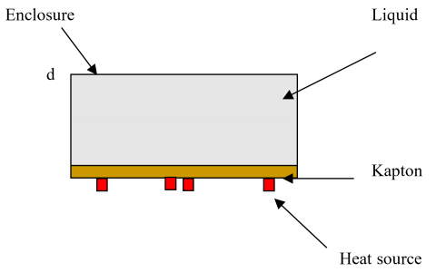
The physical model, illustrated in figure 4, is constituted by an enclosure filled with a liquid. The sensor is constituted by eight resistances printed between two polyimide sheets (Kapton). These resistances are distributed on two inside and outside strips. All the resistances are symmetrically switched for an equal-resistance Wheatstone bridge. These strips are modeled as heat sources (Figure 4). Transient models are chosen to monitor the transient thermal responses. In this numerical study, we simulate only the conduction heat transfer. The convection and radiation are neglected given that the temperature gradient is less than 1K and the thickness of resistances are very small than of liquid. Moreover, the heating time is small. To ensure the accuracy of calculations, convergence criteria is set to 10-4. The heat transfer exchanges between the system and the environment are represented by the coefficients h. In this case, the viscous dissipation and the compression forces are neglected.
Figure 4. Physical model
Due to the sufficient length of the strips, the heat losses at both ends are negligible. For this reason, the three-dimensional heat conduction model can be limited to two spatial dimensions. Therefore, the heat conduction equation may be defined in a cross-sectional area perpendicular to the strips. The numerical integration domain can be reduced to a quarter of the cross-sectional area due to the symmetrical setup.
The governing equation of the 2D axial symmetry unsteady heat conduction problem is given by [18]:
$∇(l_i ∇T_i )=ρ_i C_{pi}\frac{∂T_i}{∂t}$ (12)
where i is the material layer.
Coupled with initial and boundary conditions:
$T(t=0)=T_0$
$-\lambda\frac{∂T}{∂x}=h(T-T_0 ) x=l, y∈[0, d], x∈[0,l], y=d$
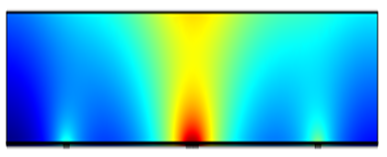
The problem is solved using a finite element method. A domain of interest is represented as an association of finite elements. Approximating functions in finite elements are determined in terms of nodal values. The continuous physical problem is then converted into a discretized finite element problem with unknown nodal values. In the case of a linear problem, a system of linear algebraic equations is obtained. The obtained linear system is solved with step time of Δt=10-3 s. An example of the obtained temperature distribution is represented on Figure 5.
Figure 5. Distribution of temperature
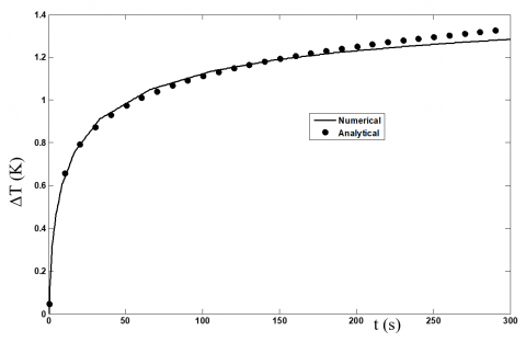
The temperature is calculated using the analytical and the numerical models. Figure 6 represents a comparison between obtained values. It can be seen that the analytical and the simulation curves fit greatly. These comparisons verify the validity of the numerical settings.
Figure 6. Comparison between numerical and analytical models
The experimental setup illustrated in Figure 7 is constituted by a cell filled with liquid. The sensor, placed in this cell, is connected with a current generator and an Agilent acquisition card. The recorded signal from the output of the Agilent card is transferred to a computer using the RS 232 serial interface. The sensor, constituted by eight resistances, has the following dimensions 120×60×0.055 mm3. All the resistances are symmetrically switched for an equal-resistance Wheatstone bridge. As long as the sample temperature is uniformed, the bridge is inherently balanced. A constant current is passed through the bridge to heat the resistances, thus resulting in unbalancing of the bridge due to the resistance change. The input Vin and output Vout voltages are measured using a computerized data acquisition system (Agilent card). The sensor system has been fabricated in such a way that the data acquisition system can be easily connected and disconnected for measurement. The bridge voltage output and the acquisition time are measured and stored simultaneously. Post-processing of the acquired data is then performed in order to calculate the resistance change, temperature change and then the thermal conductivity of the test fluid.
Figure 7. Experimental setup
In order to investigate the performance of the presented setup, different liquids have been analysed. Measurements are performed on water, starch-water mixture (volume fraction of water 0.75), mineral oil, olive oil, engine oil, ethanol and ethylene glycol samples. The current values supplied to the sensor are about 200 mA and 150 mA relatively for a duration of 25s. The acquisition time step used in all experiments is 0.1s. At each temperature, five individual tests were carried out to check the repeatability of the measurement results.
Figure 8 shows an example of the output signal of the sensor. This figure illustrates the variation of tension versus acquisition time. In order to calculate the instantaneous slope, the sensor output signal is represented versus time logarithm (Figure 9).
For each material, we made a series of measurements of the thermal conductivity and studied the distribution of the measured values. The thermal conductivity is calculated from the maximum slope using Eq. (11). Then, mean value is calculated and the obtained results at 300 K are presented in Table (1). The relative uncertainty is calculated using the same equation.
From Table 1, one can see that the thermal conductivity is measured with high accuracy; the relative uncertainty is relatively less than 4 % expect for water, it is about 5.6 %. The comparison of these relative uncertainties allows us to confirm the fact that the measurement of the thermal conductivity for water is slightly less precise than for other liquids. This is due to the presence of air bubbles in water which make some problems essentially for the measurement with the sensor. These air bubbles may cause errors in the measurement of the thermal parameters as the thermal heat transfer is reduced locally into the fluids.
Figure 8. Sensor output signal versus time
Figure 9. Sensor output signal versus time logarithm
The measurement results are compared with values given in the literature. From Table (2), we remark a good agreement between our experimental measurements and the data indicated in the literature.
Table 1. Illustration of the average thermal conductivities measured for different liquids
|
|
Sensor values |
Relative uncertainty |
|
Water |
0.585 |
5.6 % |
|
Starch-water mixture |
0.528 |
1.3 % |
|
Distilled water |
0.566 |
2.2% |
|
Mineral oil |
0.135 |
3.8 % |
|
Engine oil |
0.145 |
1.4% |
|
Olive oil |
0.165 |
2% |
|
Ethanol |
0.182 |
1.5% |
|
Ethylene glycol |
0.250 |
3% |
Table 2. Comparison between sensor measurements and literature values
|
|
Sensor values |
Literature values |
|
Water |
0.585 |
0.599 [21] |
|
Starch-water mixture |
0.528 |
0.535 [22] |
|
Distilled water |
0.566 |
0. 565 [23] |
|
Mineral oil |
0.135 |
0.130 [24] |
|
Engine oil |
0.145 |
0.145 [6, 25] |
|
Olive oil |
0.165 |
0.170 [24] |
|
ethanol |
0.182 |
0.187 [24] |
|
Ethylene glycol |
0.250 |
0.253 [21, 22] |
The ideal model assumes that the fluid properties, such as heat capacity, density, viscosity and thermal conductivity are constant. But in the real experimental process, they will change with the increase of the fluid temperature depending on the temperature coefficients of each property. This will influence the measurement results. The main problems come from the compressibility of fluids and the finite cell dimensions. In our case, the increase of temperature by the sensor is small, so we can neglect the corrections induced by properties variation.
When the temperature of the sensor increases, part of the thermal energy can be transferred into the fluid and its surroundings by thermal radiation, which reduces the energy transferred by heat conduction. In our case, the temperature rise is too small, so the effect of radiation can be unimportant.
We can conclude from the measurements presented above that our device proves to give coherent values of the thermal conductivity.
Throughout this paper, we have presented an electrothermal method for measuring the thermal conductivity of liquids. It is based on a Wheatstone bridge constituted by four tandem strips on foil sensor. Numerical model is compared to analytical one and the thermal conductivity is calculated using the instantaneous slope of the sensor output signal. The obtained results are estimated with small relative uncertainty and show a good agreement with literature data. Then, our method proves to be very practical for the measurement of thermal characteristics of materials used in various technological fields such as biology and nanofluids.
The authors wish to thank the Physikalish-Technische Bundesanstalt, Braunschweig, Germany, and especially Mr. Vladislav Meier and Dr. Ulf Hammerschmidt for providing the THB sensors used in this study and for their valuable information about the method.
|
a |
thermal diffusivity (m2s-1) |
|||
|
c |
heat capacity (J kg-1 K-1) |
|||
|
Di |
distance between sensor strips (m) |
|||
|
Nu |
local Nusselt number along the heat source |
|||
|
IB |
sensor current (A) |
|||
|
Leff |
effective strip length (m) |
|||
|
LL |
length of the long sensor resistance (m) |
|||
|
Ls |
length of the short sensor resistance (m) |
|||
|
mi |
reduced instantaneous slope |
|||
|
q |
linear heat flux density (W m-1) |
|||
|
Reff |
effective sensor electrical resistance (Ω) |
|||
|
Ri |
electrical resistance of a striplet (Ω) |
|||
|
T |
temperature (K) |
|||
|
t |
time (s) |
|||
|
Ta |
ambient temperature (K) |
|||
|
UB |
sensor output signal (V) |
|||
|
Greek symbols |
||||
|
ρ |
density (kg m-3) |
|||
|
l |
thermal conductivity (Wm-1K-1) |
|||
[1] Le Neindre B. (1996). Mesure de la conductivité thermique des liquides et des gaz. in: Techniques de l’Ingénieur, Mesures et contrôle (Tech. ing., Mes.contrôle), RC3, noR2920 R2920.1–R2920.21.
[2] Parker WJ, Jenkins RJ, Butler CP, Abbot GL. (1961). Flash method of determining thermal diffusivity, heat capacity and thermal conductivity. Journal of Applied Physics 32(9): 1679-0. http://dx.doi.org/10.1063/1.1728417
[3] Schriempf JT. (1972). A laser flash technique for determining thermal diffusivity of liquid metals at elevated temperatures. Review of Scientific Instruments 43(5): 781. http://dx.doi.org/10.1063/1.1685757
[4] Farooq MM, Giedt WH, Araki N. (1981). Thermal diffusivity of liquids determined by flash heating of a three-layered cell. International Journal of Thermophysics 2(1): 39-54. http://dx.doi.org/10.1007/BF00503573
[5] Remy B, Degiovanni A. (2005). Parameters estimation and measurement of thermophysical properties of liquids. International Journal of Heat and Mass Transfer 48: 4103-4120. http://dx.doi.org/10.1016/j.ijheatmasstransfer.2005.03.004
[6] Remy B, Degiovanni A. (2008). Measurements of the thermal conductivity and thermal diffusivity of liquids. Part II: Convective and radiative effects. International Journal of Thermophysics 27: 949-969. http://dx.doi.org/10.1007/s10765-006-0067-9
[7] Coquard R, Panel B. (2009). Adaptation of the FLASH method to the measurement of the thermal conductivity of liquids or pasty materials. International Journal of Thermal Sciences 48(4): 747-760. https://doi.org/10.1016/j.ijthermalsci.2008.06.005
[8] Forero-Sandoval IY, Pech-May NW, Alvarado-Gil JJ. (2018). Measurement of the thermal transport properties of liquids using the front face flash method. Infrared Physics and Technology 93: 9–15. http://dx.doi.org/10.1016/j.infrared.2018.07.009
[9] Blackwell JH. (1954). A transient-flow method for determining thermal constants of insulating materials in bulk. Journal of Applied Physics 25(2): 137-144. http://dx.doi.org/10.1063/1.1721592
[10] Fan J, Zhu ZX, XP Wang, Song FH, Zhang LH. (2018). Experimental studies on the liquid thermal conductivity of three saturated fatty acid methyl esters components of biodiesel. The Journal of Chemical Thermodynamics 125: 200–204. http://dx.doi.org/10.1016/j.jct.2018.06.005
[11] Azarfar SH, Movahedirad S, Sarbanha AA, Norouzbeigi R, Beigzadeh B. (2016). Low cost and new design of transient hot-wire technique for the thermal conductivity measurement of fluids. Applied Thermal Engineering 105: 142-150. http://dx.doi.org/10.1016/j.applthermaleng.2016.05.138
[12] Kwon SY, Lee SY. (2012). Precise measurement of thermal conductivity of liquid over a wide temperature range using a transient hot-wire technique by uncertainty analysis. Thermochimica Acta 542: 18-23. http://dx.doi.org/10.1016/j.tca.2011.12.015
[13] Murshed SMS, Leong KC, Yang C. (2005). Enhanced thermal conductivity of TiO2-water based nanofluids. International Journal of Thermal Sciences 44: 367-373. http://dx.doi.org/10.1016/j.ijthermalsci.2004.12.005
[14] Bhattacharya A, Mahajan RL. (2003). Temperature dependence of thermal conductivity of biological tissues. Physiological Measurement 24: 769-783. http://dx.doi.org/10.1088/0967-3334/24/3/312
[15] Santos WND, Gregorio R. (2002). A nonlinear least‐squares fitting method was employed in the calculations. J. Appl. Polym. Sci 85: 1779-1786.
[16] Murshed SMS, Leong KC, Yang C. (2006). Determination of the effective thermal diffusivity of nanofluids by the double hot-wire technique. J. Phys. D: Appl. Phys 39: 5316-5322. http://dx.doi.org/10.1088/0022-3727/39/24/033
[17] Xie H, Gu H, Fujii M, Zhang X. (2006). Short hot wire technique for measuring thermal diffusivity of various materials. Meas. Sci. Technol 17: 208-214. http://dx.doi.org/10.1088/0957-0233/17/1/032
[18] Gustafsson SE. (1987). Transient hot strip techniques for measuring thermal conductivity and thermal diffusivity. Rigaku J. 4: 16-28. http://dx.doi.org/10.1088/0022-3727/12/9/003
[19] Hammerschmidt U, Meier V. (2006). New Transient Hot-Bridge Sensor to Measure Thermal Conductivity. Thermal Diffusivity, and Volumetric Specific Heat, Int. J. thermophys. 27(3): 840-865. http://dx.doi.org/10.1007/s10765-006-0061-2
[20] Faouel J, Mzali F, Ben Nasrallah S. (2012). Thermal conductivity and thermal diffusivity measurements of wood in the three anatomic directions using the transient hot-bridge method. Special Topics & Reviews in Porous Media: An International Journal 3(3): 229-237. https://doi.org/10.1615/SpecialTopicsRevPorousMedia.v3.i3.50
[21] Kuntner J, Chabicovsky R, Jakoby B. (2005). Sensing the thermal conductivity of deteriorated mineral oils using a hot-film microsensor. J Sensors and Actuators 123: 397-402. https://doi.org/10.1016/j.sna.2005.02.041
[22] Morley MJ, Miles CA. (1997). Modelling the thermal conductivity of starch–water gels. Journal of Food Engineering 33: l-14. http://dx.doi.org/10.1016/s0260-8774(97)00043-5
[23] Angue Mintsa H, Roy G, Tam Nguyen C, Doucet D. (2009). New temperature dependent thermal conductivity data for water-based nanofluids. International Journal of Thermal Sciences 48: 363-371. http://dx.doi.org/10.1016/j.ijthermalsci.2008.03.009
[24] Huang L, Liu L. (2009). Simultaneous determination of thermal conductivity and thermal diffusivity of food and agricultural materials using a transient plane-source method. Journal of Food Engineering 95: 179-185. http://dx.doi.org/10.1016/j.jfoodeng.2009.04.024
[25] Wang XQ, Arun SM. (2007). Heat transfer characteristics of nanofluids: A review. International Journal of Thermal Sciences 46: 1-19. http://dx.doi.org/10.1016/j.ijthermalsci.2006.06.010