Noureddine Fares* | Zoubir Aoulmi | Tawfik Thelaidjia | Djamel Ounnas
© 2022 IIETA. This article is published by IIETA and is licensed under the CC BY 4.0 license (http://creativecommons.org/licenses/by/4.0/).
OPEN ACCESS
Induction machine health monitoring is considered a developing technology for the online detection of faults that occur even at the initial stage. The objective of this study is to present an artificial intelligence (AI) technique for the detection and localization of adjacent and distant broken bar faults in the induction machine, through a multi-winding model for the simulation of these cases. In this work, it was found that the application of Artificial Neural Networks (ANN) based on Mean Squared Error (MSE) and Random Forest (decision tree) plays an important role in detecting and locating defaults. The stator current signal Ias of a motor in the dynamic state was acquired from a healthy and faulty motor with a broken rotor bar fault. 9 statistical features and 8 wavelet packet parameters are extracted from the stator current signal. These features were employed as an input vector to train and test the ANN and random fores29t and determine whether the motor was running under normal conditions or defective. For optimizing the rotor bar defect classification procedure, feature selection algorithms are adopted, such as BBAT and BPSO. For feature reduction, we used the principal component analysis (PCA) algorithm, to reduce the number of features. The results showed that the random forest classifier based on statistical parameters and wavelet packet parameters followed by PCA can detect the defective with high accuracy (98.3333%) compared to other methods.
induction motor health monitoring, (BPSO, BBAT and PCA) optimization algorithms, broken rotor bar, statistical features, wavelet packet transform (WPT), random forest (RF), artificial neural network (ANN)
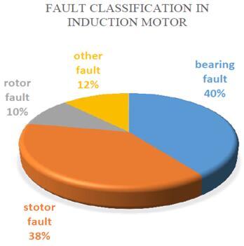
Fault diagnostic induction motors are a component of many industrial process applications, due to their robustness, cost and performance. They are used in various applications as a means of energy conversion, pumps, electric vehicles, and asynchronous generators. Significant defects in electrical machinery (Figure 1); Bhasme and Chavhan [1] can be broadly classified as follows: stator defects, broken rotor bar, and bearing defects are the most common [2].
Figure 1. Fault classification of induction motor
In this context, over the past two decades, the diagnosis of induction machine failures has aroused great interest on the part of researchers. Major research has been carried out for the development of various techniques and methods for detecting and diagnosing defects. He proposed an algorithm for the online detection of rotor bar rupture in induction machines based on the use of wavelet packet decomposition and neural networks [3]. A new set of characteristic coefficients is obtained by the WPD of the stator current, to build a neural network for defect detection, thus accurately differentiating healthy and defective conditions. The algorithm analyzes rotor bar defects by WPD of the stator current of the induction motor. In the study [4], a defect diagnosis technique for induction machines under rotor and stator failures is carried out, taking into account the harmonic components in the current signal. This diagnostic method is carried out using the MCSA method. The sideband components of the current spectrum are extracted and analyzed to prove rotor defects. The article [5] focuses on improving a new fault classification technique using support vector machines (SVMs) for induction motors. Several defects of the induction machine, such as a BRB, an unbalanced phase defect, and an unbalanced rotor, are examined. Based on a three-phase model of the time domain, the BRB with various conditions was simulated to examine the resulting torque-velocity characteristic in each condition. The advanced defect diagnosis system can recognize the type of BRB defects in the squirrel cage induction motor [6-8].
In this work, a multi-winding model is presented to simulate the behavior of the machine is healthy and defective cases when the rotor bar is broken, defect diagnosis is based on an intelligent artificial technique (AI) very important for the detection of a rotor defect in the induction machine. The identification process shows a sequence of simulation configuration, data acquisition, data processing, classification algorithm, model evaluation, and last prediction. In the fifth section, the application of the ANN and RF configuration based on the learning machine is proposed to take the data set for machine training purposes. The training dataset is taken for five failure conditions and one health condition. The defect condition is adjacent and distant broken rotor bars. This drive dataset is used to train the machine using three algorithms BAT, BPSO, PCA, and without optimization. Each algorithm shows a different accuracy for the defect identification method proposed in the sixth section (Table 4). The highest test accuracy classification of healthy or broken rotor bars of the induction machine is obtained by random forest (RF) with the hybrid parameter used by PCA (statistical and wavelet packet parameters) is (98.3333%).
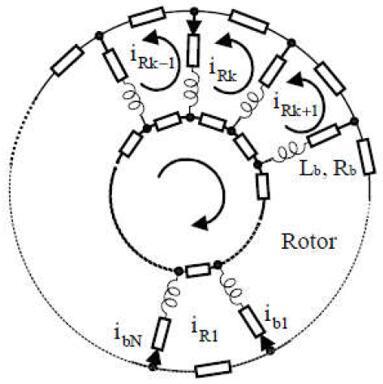
To be able to focus on the study of the simulation of bar break defects, a model of the rotor is established in the form of electrically connected and magnetically coupled meshes, where a mesh consists of two bars and the two portions of rings that connect them. Each bar and ring segment is characterized by resistance and inductance (Figure 2). The model assumptions are:
Although a sinusoidal mmf of the stator winding is assumed, other winding distributions could also be analyzed by simply using superposition. This is justified by the fact that different space harmonic components do not interact [9, 10].
Figure 2. Rotor cage equivalent circuit
2.1 Equation model
By using the Clark transformation to go from three-phase stator quantities (a, b, c) to two-phase quantities (α, β). The simulation can be performed with two separate frames for the stator and the rotor. To reduce the calculation time, we eliminate the angle "ɵ" of the coupling matrix by choosing the most appropriate reference and which is that of the rotor.
In this frame, all the quantities have a pulsation "gωs" in steady-state. This characteristic can be used for the analysis of the rupture of rotor bars in the machine by observing the current "Ias" [2].
We are therefore looking for the set of independent differential equations defining the model of the induction machine.
2.1.1 Stator voltage equation
All the stator phases voltages in matrix form and flux equations are deduced [11]:
$\left[V_{a b c s}\right]=\left[R_s\right]\left[I_{a b c s}\right]+\frac{d}{d t}\left[\emptyset_{a b c s}\right]$ (1)
$\left[\emptyset_{a b c s}\right]=\left[L_s\right]\left[I_{a b c s}\right]+\left[M_{s r}\right]\left[I_{r k}\right]$ (2)
where, [Vabcs]=[Vas Vbs Vcs]T is the stator voltage vector, [Iabcs]=[Ias Ibs Ics]T is the stator current vector, [Irk]=[Ir0 Ir1 … Irk… Ir(Nr-1)]T is the vector of the currents in the rotor mesh and $\left[\emptyset_{a b c s}\right]=\left[\emptyset_{a s} \emptyset_{b s} \emptyset_{c s}\right]^T$ is the stator flux vector.
We, therefore, write the matrices of the resistances, the inductances, and the stator mutuals respectively:
$\left[R_s\right]=\left[\begin{array}{ccc}R_s & 0 & 0 \\ 0 & R_s & 0 \\ 0 & 0 & R_s\end{array}\right] ; \quad\left[L_s\right]=\left[\begin{array}{ccc}L_s & M_s & M_s \\ M_s & L_s & M_s \\ M_s & M_s & L_s\end{array}\right] ;$
$\left[M_{s r}\right]=\left[\begin{array}{ccc}\cdots & -M_{s r} \cos (\theta+k \alpha) & \cdots \\ \cdots & -M_{s r} \cos \left(\theta+k \alpha-\frac{2 \pi}{3}\right) & \cdots \\ \cdots & -M_{s r} \cos \left(\theta+k \alpha-\frac{4 \pi}{3}\right) & \cdots\end{array}\right]$
With:
$K=0,1,2, \ldots,\left(N_r-1\right)$.
$M_{s r}=\frac{4 \mu_0 N_s R l}{e p^2 \pi} \sin \left(\frac{\alpha}{2}\right) ;[H]$.
$\alpha=\frac{2 \pi}{N_r} ;[\mathrm{rad}]$.
where, Nr is the number of rotor bars, Msr is the mutual inductance between stator phase and rotor mesh and α is the angle between the rotor bars.
The transition to two-phase components of the stator components is carried out using the Park transformation matrix, knowing that the homopolar component is zero.
$\left[X_{\alpha \beta s}\right]=[P(\theta)]\left[X_{d q s}\right]$ (3)
where, $P(\theta)=\left[\begin{array}{cc}\cos (\theta) & -\sin (\theta) \\ \sin (\theta) & \cos (\theta)\end{array}\right]$, P(θ): Park's rotation matrix is as follows.
$\emptyset_{\alpha \beta s}=\left[\begin{array}{cc}L_{s c} & 0 \\ 0 & L_{s c}\end{array}\right] \cdot\left[I_{\alpha \beta s}\right]-M_{s r} \cdot\left[\begin{array}{cc}\ldots \cos (\theta+k \alpha) \ldots \\ \ldots \sin (\theta+k \alpha) \ldots\end{array}\right] \cdot\left[I_{r k}\right]$ (4)
With: Lsc=Lsp-Ms+Lsf; [H]; $L_{s p}=\frac{4 \mu_0 N_s^2 R l}{e \pi p^2} ;[H]$; $M_s=-\frac{L_{s p}}{2} ;[H]$; $\mu_0=4 \pi 10^{-7} ;\left[H . m^{-1}\right]$.
where, Lsc is the inductance cyclique statorique, Lsp is the main inductance of a stator phase, Ms is the mutual between two stator windings and μ0 is the magnetic air permeability.
So, the flux and the stator voltage in the Park reference (d, q) are written respectively:
$\emptyset_{d q s}=\left[\begin{array}{cc}L_{s c} & 0 \\ 0 & L_{s c}\end{array}\right] \cdot\left[I_{d q s}\right]-M_{s r} \cdot\left[\begin{array}{ll}\ldots \cos (k \alpha)\ldots \\ \ldots \sin(k \alpha)\ldots\end{array}\right] \cdot\left[I_{r k}\right]$ (5)
$V_{d q s}=R_s \cdot I_{d q s}+\omega \cdot P\left(\frac{\pi}{2}\right) \cdot \emptyset_{d q s}+\frac{d}{d t} \emptyset_{d q s}$ (6)
After transformation and rotation, the electric equations in the rotor reference are written:
$\left\{\begin{array}{l}V_{d s}=R_s \cdot I_{d s}-\omega \cdot \emptyset_{q s}+\frac{d}{d t} \emptyset_{d s} \\ V_{q s}=R_s \cdot I_{q s}+\omega \cdot \emptyset_{d s}+\frac{d}{d t} \emptyset_{q s}\end{array}\right.$ (7)
Finally, the electrical equation of the stator in the rotor frame is written in matrix form:
$\left[\begin{array}{c}V_{d s} \\ V_{q s}\end{array}\right]=\left[\begin{array}{cccc}R_s & -\omega \cdot L_{s c} & \vdots \cdots+\omega \cdot M_{s r} \cdot \sin (k \alpha) \ldots \\ \omega \cdot L_{s c} & R_s & \vdots \cdots-\omega \cdot M_{s r} \cdot \cos (k \alpha) \ldots\end{array}\right] \cdot\left[\begin{array}{c}I_{d q s} \\ I_{r k}\end{array}\right]$
$+\left[\begin{array}{ccc}L_{s c} & 0 & \vdots \cdots-M_{s r} \cdot \cos (k \alpha) \ldots \\ 0 & L_{s c} & \vdots \cdots-M_{s r} \cdot \sin (k \alpha) \ldots\end{array}\right] \cdot \frac{d}{d t}\left[\begin{array}{c}I_{d q s} \\ I_{r k}\end{array}\right]$ (8)
2.1.2 Rotor voltage equation
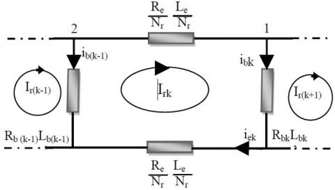
Figure 3 represents the equivalent electric circuit of a mesh of the rotor cage, where the rotor bars and the portions of short-circuit rings are represented by their resistances and corresponding leakage inductances [12].
Figure 3. Electric diagram equivalent of a rotor mesh
Knowing that:
$\left\{\begin{array}{c}I_{e k}=I_{r k}-I_e \\ I_{b k}=I_{r k}-I_{r(k+1)}\end{array}\right.$ (9)
The voltage equation for a mesh "k" of the rotor cage is given by:
$-R_{b(k-1)} I_{r(k-1)}+R_{b k} I_{b k}+\frac{R_e}{N_r} I_{e k}+\frac{R_e}{N_r} I_{r k}+\frac{d}{d t} \emptyset_{r k}=0$ (10)
The total flux "$\emptyset_{r k}$" for an elementary circuit of index "k" is composed of the sum of the following terms:
Main flux: Lrp.Irk;
Mutual flux with the other circuits of the rotor:
$M_{r r} \cdot \sum_{\substack{j=0 \\ j \neq k}}^{N_r-1} I_{r j}$
Mutual flux with the stator, given after transformation:
$-\frac{3}{2} M_{s r} \cdot\left[\begin{array}{ccc}\vdots & \vdots & \vdots \\ \cos (k \alpha) & \vdots & \sin (k \alpha) \\ \vdots & \vdots & \vdots\end{array}\right] \cdot\left[I_{d q s}\right]$
The flux induced in the rotor mesh is given by:
$\emptyset_{r k}=\left(L_{r p}+2 L_b+2 \frac{L_e}{N_r}\right) I_{r k}+M_{r r} \cdot \sum_{\substack{j=0 \\ j \neq k}}^{N_r-1} I_{r j}-L_b\left(I_{r(k-1)}+I_{r(k+1)}\right)$
$-\frac{3}{2} M_{s r}\left(I_{d s} \cos (k \alpha)+I_{q s} \sin (k \alpha)\right)-\frac{L_e}{N_r} I_e$ (11)
It is finally necessary to complete the system of the equation of the circuits of the rotor by that of the ring of short-circuits; we then have:
$\frac{R_e}{N_r} \sum_{k=0}^{N_r-1} I_{r k}+\frac{L_e}{N_r} \sum_{k=0}^{N_r-1} \frac{d I_{r k}}{d t}-R_e I_e-L_e \frac{d I_e}{d t}=0$ (12)
with: $L_{r p}=\frac{2 \pi\left(N_r-1\right) \mu_0 R l}{e N_r^2} ;[H]$; $M_{r r}=-\frac{2 \pi \mu_0 R l}{e N_r^2} ;[H]$.
where, Lrp is the main inductance of a rotor mesh, Mrr is the mutual inductance between adjacent, Irk is the mesh current "k” and Ie is the short-circuit ring current.
The complete system is:
$\left[\begin{array}{c}V_{d s} \\ V_{q s} \\ 0 \\ \vdots \\ 0\end{array}\right]=[L] \cdot \frac{d}{d t}\left[\begin{array}{c}I_{d s} \\ I_{q s} \\ \vdots \\ I_{r k} \\ \vdots\end{array}\right]+[R]\left[\begin{array}{c}I_{d s} \\ I_{q s} \\ \vdots \\ I_{r k} \\ \vdots\end{array}\right]$ (13)
So, becomes:
2.2 Equivalent reduced model of the induction machine
The representation of the state shows a very high order system because it consists of the number of phases of the stator, the number of phases of the rotor, and the electromechanical equations. The rank of the system is, therefore "Nr+3". It is therefore necessary to reduce the size of the matrices to reduce the simulation time [13].
To do this, we use the generalized Clarke matrix extended to the rotor system. This makes it possible to move from "n-phases" modeling to equivalent two-phase modeling written as follows [14]:
The electromagnetic torque is obtained by derivation of the co-energy:
$C_{e m}=\frac{3}{2} p\left[I_{d q s}\right]^T \frac{\delta}{\delta \theta}\left[\begin{array}{ccc}\cdots & -M_{s r} \cos (\theta+k \alpha) & \cdots \\ \cdots & -M_{s r} \sin (\theta+k \alpha) & \cdots\end{array}\right]\left[\begin{array}{c}\vdots \\ I_{r k} \\ \vdots\end{array}\right]$ (15)
$C_{e m}=\frac{3}{2} p M_{s r}\left\{I_{d s} \sum_{k=0}^{N_r-1} I_{r k} \sin (k \alpha)-I_{q s} \sum_{k=0}^{N_r-1} I_{r k} \cos (k \alpha)\right\}$ (16)
We add the mechanical equation to have the mechanical speed "Ω=ω/P”.
$\frac{d \Omega}{d t}=\frac{1}{J} p\left(C_{e m}-C_r-\frac{f}{p} \omega\right)$ (17)
with: $\frac{d \theta}{d t}=\omega$.
$\left[T_{3 n}\left(\theta_r\right)\right]=\frac{2}{n} \cdot \left[\begin{array}{ccccc}\frac{1}{2} & \cdots & \cdots & \cdots & \frac{1}{2} \\ \cos \left(\theta_r\right) & \cdots & \cos \left(\theta_r-k p \frac{2 \pi}{n}\right) & \cdots & \cos \left(\theta_r-(n-1) p \frac{2 \pi}{n}\right) \\ -\sin \left(\theta_r\right) & \cdots & -\sin \left(\theta_r-k p \frac{2 \pi}{n}\right) & \cdots & -\sin \left(\theta_r-(n-1) p \frac{2 \pi}{n}\right)\end{array}\right]$ (18)
The inverse matrix is given by:
$\left[T_{3 n}\left(\theta_r\right)\right]^{-1}=\left[T_{n 3}\left(\theta_r\right)\right]=\left[\begin{array}{ccc}1 & \cos \left(\theta_r\right) & -\sin \left(\theta_r\right) \\ \vdots & \vdots & \vdots \\ \vdots & \cos \left(\theta_r-k p \frac{2 \pi}{n}\right) & -\sin \left(\theta_r-k p \frac{2 \pi}{n}\right) \\ 1 & \vdots & \vdots \\ & \cos \left(\theta_r-(n-1) p \frac{2 \pi}{n}\right) & -\sin \left(\theta_r-(n-1) p \frac{2 \pi}{n}\right)\end{array}\right]$ (19)
After applying this transformation matrix, a state vector [X] is defined, will give:
$\left\{\begin{array}{c}{\left[X_{0 d q s}\right]=\left[T\left(\theta_s\right)\right] \cdot\left[X_{a b c s}\right] \Leftrightarrow} \\ {\left[X_{a b c s}\right]=\left[T\left(\theta_s\right)\right]^{-1} \cdot\left[X_{0 d q s}\right]} \\ {\left[X_{0 d q r}\right]=\left[T_{3 N_r}\left(\theta_r\right)\right] \cdot\left[X_{r k}\right] \Leftrightarrow} \\ {\left[X_{r k}\right]=\left[T_{3 N_r}\left(\theta_r\right)\right]^{-1} \cdot\left[X_{0 d q r}\right]}\end{array}\right.$ (20)
• For the following part of the stator voltages:
$\left[V_{a b c s}\right]=\left[R_s\right]\left[I_{a b c s}\right]+\frac{d}{d t}\left\{\left[L_s\right] \cdot\left[I_{a b c s}\right]\right\}+\frac{d}{d t}\left\{\left[M_{s r}\right] .\left[I_{r k}\right]\right\}$ (21)
Applying the generalized equation to equation (21) gives:
$\left[V_{0 d q s}\right]=\left\{\left[T\left(\theta_s\right)\right] \cdot\left[R_s\right] \cdot\left[T\left(\theta_s\right)\right]^{-1}\right\} \cdot\left[I_{0 d q s}\right]+$
$\left\{\left[T\left(\theta_s\right)\right] .\left[L_s\right] .\left[T\left(\theta_s\right)\right]^{-1}\right\} \cdot \frac{d}{d t}\left[I_{0 d q s}\right]+$
$\left\{\left[T\left(\theta_s\right)\right] \cdot\left[M_{s r}\right] \cdot\left[T_{3 N_r}\left(\theta_r\right)\right]^{-1}\right\} \cdot \frac{d}{d t}\left[I_{0 d q r}\right]$ (22)
• For the rotor part:
$\left[V_{a b c r}\right]=\left[R_r\right]\left[I_{r k}\right]+\frac{d}{d t}\left\{\left[L_r\right] .\left[I_{r k}\right]\right\}+\frac{d}{d t}\left\{\left[M_{s r}\right] .\left[I_{a b c s}\right]\right\}$ (23)
$\left[V_{0 d q r}\right]=\left\{\left[T\left(\theta_r\right)\right] \cdot\left[R_r\right] \cdot\left[T_{3 N_r}\left(\theta_r\right)\right]^{-1}\right\} \cdot\left[I_{0 d q r}\right]+$
$\left\{\left[T\left(\theta_r\right)\right] \cdot\left[L_r\right] \cdot\left[T_{3 N_r}\left(\theta_r\right)\right]^{-1}\right\} \cdot \frac{d}{d t}\left[I_{0 d q r}\right]+$
$\left\{\left[T\left(\theta_r\right)\right] \cdot\left[M_{s r}\right] \cdot\left[T\left(\theta_r\right)\right]^{-1}\right\} \cdot \frac{d}{d t}\left[I_{0 d q s}\right]$ (24)
By choosing a referential linked to the rotor such that "θs=θ et θr=0". This change of landmark makes it possible to obtain, after simplification, a reduced-size model of the asynchronous machine [15]:
$\left[\begin{array}{ccccc}L_{s c} & 0 & -\frac{N_r}{2} M_{s r} & 0 & 0 \\ 0 & L_{s c} & 0 & -\frac{N_r}{2} M_{s r} & 0 \\ -\frac{3}{2} M_{s r} & 0 & L_{r c} & 0 & 0 \\ 0 & -\frac{3}{2} M_{s r} & 0 & L_{r c} & 0 \\ 0 & 0 & 0 & 0 & L_e\end{array}\right] \cdot \frac{d}{d t}\left[\begin{array}{c}I_{d s} \\ I_{q s} \\ I_{d r} \\ I_{q r} \\ I_e\end{array}\right] =\left[\begin{array}{c}V_{d s} \\ V_{q s} \\ V_{d r} \\ V_{q r} \\ V_e\end{array}\right]-\left[\begin{array}{ccccc}R_s & -L_{s c} \omega & 0 & \frac{N_r}{2} M_{s r} \omega & 0 \\ L_{s c} \omega & R_s & -\frac{N_r}{2} M_{s r} \omega & 0 & 0 \\ 0 & 0 & R_r & 0 & 0 \\ 0 & 0 & 0 & R_r & 0 \\ 0 & 0 & 0 & 0 & R_e\end{array}\right] \cdot\left[\begin{array}{c}I_{d s} \\ I_{q s} \\ I_{d r} \\ I_{q r} \\ I_e\end{array}\right]$ (25)
with: $\left\{\begin{array}{c}L_{r c}=L_{r p}-M_{r r}+\frac{2 \cdot L_e}{N_r}+2 \cdot L_b(1-\cos (\alpha)) \\ \quad R_r=2 \frac{R_e}{N_r}+2 \cdot R_b(1-\cos (\alpha))\end{array}\right.$.
After establishing the model of the squirrel-cage asynchronous machine (Table 1) considering the structure of the rotor without fault, we now proceed to the modeling of the machine taking into account the rotor fault of the bar break type.
Modeling this type of failure can be done using two different methods to cancel the current passing through the faulty bar. The first modeling method is to completely reconstruct the electrical circuit of the rotor. In this type of approach, the failed rotor bar is removed from the electrical circuit, which requires recalculation of the [Rr] resistance and inductance [Lr] matrices of the machine. Indeed, removing a bar from the cage gives us a matrix [Rr] and [Lr] of lower rank than that developed for the healthy machine. The change in the order of the rotor matrices forces the electrical and magnetic laws of the 'k' loop to be recalculated [13, 16].
The second possible approach is to artificially increase the value of the resistance of the failed bar by a factor sufficient for the current that passes through it to be as close as possible to zero in a steady-state. Compared to the first method, the structure of the rotor electrical circuit is not modified because it is considered, in this type of modeling, that a bar break does not modify the own and mutual inductances of the rotor cage.
Therefore, modeling the partial break of the bars is possible in the latter approach, as the matrix [Rr] needs to be modified.
The rotor defect matrix is therefore written as follows:
$\left[R_{r f}\right]=\left[R_r\right]+\left[\begin{array}{ccccccc}0 & \cdots & \cdots & 0 & 0 & 0 & \cdots \\ \vdots & \vdots & \vdots & \vdots & \vdots & \vdots & \vdots \\ \vdots & \vdots & \vdots & \vdots & \vdots & \vdots & \vdots \\ \vdots & \vdots & \vdots & \vdots & \vdots & \vdots & \vdots \\ 0 & \cdots & 0 & 0 & 0 & 0 & \cdots \\ 0 & \cdots & 0 & R_{b k} & -R_{b k} & 0 & \cdots \\ 0 & \cdots & 0 & -R_{b k} & R_{b k} & 0 & \cdots \\ 0 & \cdots & 0 & 0 & 0 & 0 & \cdots \\ \vdots & \vdots & \vdots & \vdots & \vdots & \vdots & \vdots\end{array}\right]$ (26)
The new rotor resistance matrix, after transformations, becomes:
$\left[R_{r f d q}\right]=\left[T\left(\theta_r\right)\right] \cdot\left[R_{r f}\right] \cdot\left[T\left(\theta_r\right)\right]^{-1}$ (27)
So, the reduced-size model (5X5) of the induction machine with rotor bar breakage defects becomes:
$\left[\begin{array}{ccccc}L_{s c} & 0 & -\frac{N_r}{2} M_{s r} & 0 & 0 \\ 0 & L_{s c} & 0 & -\frac{N_r}{2} M_{s r} & 0 \\ -\frac{3}{2} M_{s r} & 0 & L_{r c} & 0 & 0 \\ 0 & -\frac{3}{2} M_{s r} & 0 & L_{r c} & 0 \\ 0 & 0 & 0 & 0 & L_e\end{array}\right] \cdot \frac{d}{d t}\left[\begin{array}{c}I_{d s} \\ I_{q s} \\ I_{d r} \\ I_{q r} \\ I_e\end{array}\right]= \left[\begin{array}{c}V_{d s} \\ V_{q s} \\ V_{d r} \\ V_{q r} \\ V_e\end{array}\right]-\left[\begin{array}{ccccc}R_s & -L_{s c} \omega & 0 & \frac{N_r}{2} M_{s r} \omega & 0 \\ L_{s c} \omega & R_s & -\frac{N_r}{2} M_{s r} \omega & 0 & 0 \\ 0 & 0 & R_{r d d} & R_{r d q} & 0 \\ 0 & 0 & R_{r q d} & R_{r q q} & 0 \\ 0 & 0 & 0 & 0 & R_e\end{array}\right] \cdot\left[\begin{array}{c}I_{d s} \\ I_{q s} \\ I_{d r} \\ I_{q r} \\ I_e\end{array}\right]$ (28)
with:
$R_{r d d}=2 \cdot R_b(1-\cos (\alpha))+\frac{R_e}{N_r}+\frac{2}{N_r}(1-\cos (\alpha))$.
$\sum_k R_{b f k}(1-\cos (2 k-1) \cdot \alpha)$
$R_{r d q}=-\frac{2}{N_r}(1-\cos (\alpha)) \sum_k R_{b f k} \sin (2 k-1) \cdot \alpha$
$R_{r q d}=-\frac{2}{N_r}(1-\cos (\alpha)) \sum_k R_{b f k} \sin (2 k-1) \cdot \alpha$
$R_{r q q}=2 \cdot R_b(1-\cos (\alpha))+2 \cdot \frac{R_e}{N_r}+\frac{2}{N_r}(1-\cos \alpha) \cdot \sum_k R_{b f k}(1+\cos (2 k-1) \cdot \alpha)$ (29)
The index "k" indicates the broken bar.
For the mechanical part, after application of the generalized transformation on the expression of the torque (16) is obtained:
$C_{e m}=\frac{3}{2} \cdot p \cdot \frac{N_r}{2} \cdot M_{s r} \cdot\left(I_{d s} \cdot I_{q r}-I_{q s} \cdot I_{d r}\right)$ (30)
Table 1. Induction machine parameters
|
Parameter |
Meaning parameter |
Value |
|
P |
Nominal power |
1.1 KW |
|
V |
Rated line voltage |
220 V |
|
fs |
Feeding frequency |
50 Hz |
|
p |
Number of pole pairs |
1 |
|
R |
average rotor diameter |
35.76 mm |
|
Ns |
Number of turns per stator phase |
160 |
|
l |
Rotor active length |
65 mm |
|
Re |
Resistance of a portion of a short-circuit ring |
150 μΩ |
|
Rb |
Resistance of a rotor bar |
150 μΩ |
|
Le |
Short circuit ring leakage inductance |
0.1 μH |
|
Lb |
Rotor bar leakage inductance |
0.1 μH |
|
e |
Air gap thickness |
0.2 mm |
|
Rs |
Resistance of a stator phase |
7.58 Ω |
|
Nr |
Number of rotor bars |
16 |
|
Lsf |
Stator leakage inductance |
26.5 mH |
|
f |
Coefficient of friction |
0 |
|
J |
Moment of inertia |
0.00541 Kgm2 |
2.3 Simulation results and discussion
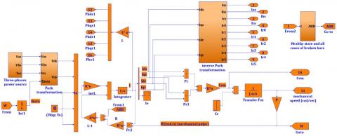
Once the model of the induction machine is established. The simulation aspect can be addressed in the MATLAB/Simulink environment, which provides the ability to observe and interpret visualized phenomena and quantities in real-time. We will represent the induction machine in different states (Figure 4), healthy and defective. The results of the simulation in these cases are as follows:
Figure 4. Simulation model of an induction machine with healthy and all cases of broken bars state
Figure 5. Three-phase supply voltage Vabcs
Figure 6. Park’s two-phase stator voltages Vdqs
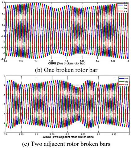
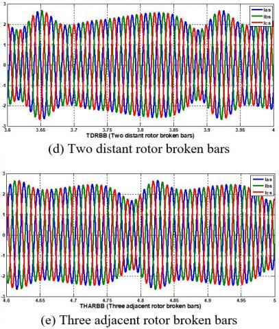
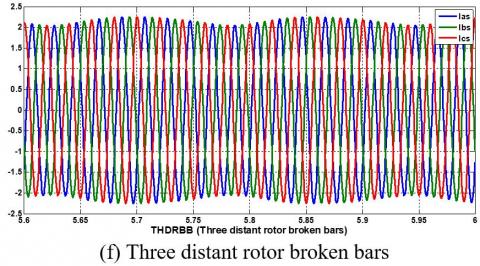
Figure 7. Three-phase stator currents Iabcs of an induction machine with the zoom of healthy and all cases of broken rotor bars state
Figure 8. FFT analysis of stator current Ias spectrum for the healthy state of the induction machine
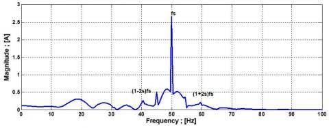
Figure 9. FFT analysis of stator current Ias spectrum for rotor broken bars of the induction machine
Figure 10. Mechanical speed of induction machine with healthy and all cases of broken rotor bars state
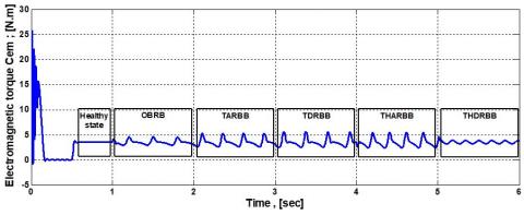
Figure 11. Electromagnetic torque of induction machine with healthy an all cases of broken rotor bars state
Observe and simulate the multi-winding model of the induction machine with three supply voltages Vabcs and Vdqs (Figure 5, 6). At the time 0.5 s, apply a load torque of 3.5; [Nm]. Before 1 s the dynamic regime of the asynchronous machine in the healthy state, the time t=1 s, simulates the rupture of the first bar, the time t=2 s, breaking two adjacent bars, and the time t=3 s, breaking two distant bars, and at time t=4 s, breaking three adjacent bars, and at time t=5 s, by breaking three distant bars, it is observed in Figure 10 that the rotational speed decreases during the break of the bar and creates oscillations of rupture. Figure 11 electromagnetic torque increases in amplitude after the rupture of two bars, and Figure 7 is illustrated the modulation of the envelope of the stator currents Iabcs increases in amplitude with the number of broken bars.
Figure 8 shows the spectral analysis of the stator current Ias through the FFT in the healthy state, we do not observe any increase in frequency. Figure 9 shows the appearance of a raised frequency for the adjacent broken bar. These increases have an amplitude that increases according to the bars of the number of breaks, two frequencies appear around the fundamental f=50 Hz, one on the left and the other on the right according to the relationship $f_{b b}=(1 \mp 2 s k) f_s$.
3.1 Statistical features
At the final stage of signal processing, the statistical characteristics of the current signal are extracted (Table 2). and used as input for ANN and RF for training to classify various signals according to the degree of similarity or manifestation of these characteristics. Each type of defect produces a signal from the stator current Ias with a signature pattern that is reflected in signal characteristics such as mean, standard deviation, etc. [17].
Table 2. Statistical features
|
statistical features |
Equation |
|
minimum |
Min(x) |
|
maximum |
Max(x) |
|
Standard deviation |
$\frac{1}{N} \sum_{i=0}^N \bar{x}_i^2-\bar{x}^2$ |
|
Root mean square |
$\frac{1}{N} \sum_{i=0}^N x_i^2$ |
|
Kurtosis |
$\frac{1}{N} \sum_{i=0}^N \bar{x}_i^4-\frac{3}{N^2}\left(\sum_{i=0}^N x_i^2\right)^2-\frac{4}{N} \bar{x}\left(\sum_{i=0}^N x_i^2\right)+\frac{12}{N} \bar{x}^2\left(\sum_{i=0}^N x_i^2\right)-6 \bar{x}^4$ |
|
peak to peak |
Max(x)-min(x) |
|
Mean |
$\frac{1}{N} \sum_{i=0}^N x_i$ |
|
Skewness |
$\frac{1}{N} \sum_{i=0}^N x_i^3-\frac{3}{N} \bar{x}\left(\sum_{i=0}^N x_i^2\right)+2 \bar{x}^3$ |
|
Crest factor |
$\frac{\max (x)-\min (x)}{\frac{1}{N} \sum_{i=0}^N x_i^2}$ |
3.2 Wavelet packet decomposition features
3.2.1 Description of the wavelet method
The wavelet method requires the use of basic time-frequency functions with different time supports to analyze signal structures of different sizes. The wavelet transforms, an extension of the short-term Fourier transform, projects the original signal onto the basic functions of the wavelets and provides time-domain mapping at the time scale.
A wavelet is a function belonging to L2(R) of zero mean. It is normalized and centered on the neighborhood of t=0. A family of time-frequency atoms is obtained by scaling a bandpass filter ψ by s and translating it as u. L2(R) represents the spatial vector of the integrable functions of the measurable square on the real line R with ‖ψ‖=1.
$\int_{-\infty}^{+\infty} \psi(t) d t=0$ (31)
$\psi_{u, s}(t)=\frac{1}{\sqrt{s}} \psi\left(\frac{t-u}{s}\right)$ (32)
The wavelet transforms a function f at scale s and the position u is calculated by correlating f with a wavelet atom:
$W_f(u, s)=\int_{-\infty}^{+\infty} f(t) \frac{1}{\sqrt{s}} \psi \cdot\left(\frac{t-u}{s}\right) d t$ (33)
A real wavelet transform is complete and conserves energy as long as it satisfies a low eligibility requirement:
$\int_0^{+\infty} \frac{|\psi(\omega)|^2}{|\omega|} d \omega=\int_{-\infty}^0 \frac{|\psi(\omega)|^2}{|\omega|} d \omega=C_\psi<+\infty$ (34)
where, Wf(u, s) is known only for s<s0, one must retrieve f, an additional information corresponding to Wf(u, s) for s>s0. This is achieved by introducing a scale function φ which is an aggregate of wavelets at scales greater than ψ.
In the following, we draw by $\hat{\psi}(\omega)$ and $\hat{\varphi}(\omega)$ the Fourier transforms of ψ(n) and φ(n), respectively.
The transformation into discrete wavelets results from the continuous version. Unlike the latter, DWT uses a discrete scale factor and translation. A discrete dyadic wavelet transform is called any wavelet base working with a scale factor u=2j.
The discrete version of Wavelet Transform, DWT, consists of sampling neither the signal nor the transform but sampling the scaling and shift parameters [18, 19].
This results in high-frequency resolution at low frequencies and high temporal resolution at high frequencies, eliminating redundant information. Taking into account the positive frequency, $\hat{\varphi}(\omega)$ has information in [0, π] and $\widehat{\psi}(\omega)$ in [π, 2π]. Therefore, they both have complete signal information without any redundancy. The functions h(n) and g(n) can be obtained by the scalar product of ψ(t) and φ(t) [20]. The decomposition of the signal into [0, π] gives:
$h(n)=<2^{-l} \varphi\left(2^{-l} t\right) \varphi(t-n)> \mathrm{g}(n)=<2^{-j} \psi\left(2^{-j} t\right) \varphi(t-n)>, j=0,1, \ldots,$ (35)
Wavelet decomposition does not involve the signal in [π, 2π]. To break down the signal throughout the frequency band, wavelet packets can be used. After decomposition l times, we obtain 2l frequency bands each with the same bandwidth either:
$\left[\frac{(i-l) f_n}{2}, \frac{i f_n}{n}\right] \quad i=1,2, \ldots, 2^l$ (36)
where, fn is the Nyquist frequency, in the ith frequency band. Wavelet packets break down the signal into a low-pass filter h(n) and (2l-1) band-pass filters g(n), and provide diagnostic information in two frequency bands. Aj is the low-frequency approximation and Dj is the high-frequency detail signal, both at j resolution:
$A_j(n)=\sum_k h(k-2 n) A_{j-1}$
$D_j(n)=\sum_k g(k-2 n) A_{j-1} \quad n=1,2, \ldots$ (37)
where, A0(k) is the original signal. After decomposition of the signal, an approximation signal Aj and detail signals Dj are obtained (see Figure 12).
Figure 12. Tree decomposition of signal S
The wavelet packet method is a generalization of wavelet decomposition that offers a richer range of possibilities for signal analysis (see Figure 13). In wavelet analysis, a signal is divided into an approximation and a detail. Then the approximation is divided into an approximation and a second-level detail, and the process is repeated [21] until the targeted results are obtained. For n-level decomposition, there are n+1 possible ways to decompose or encode the signal:
$W_{2 n}(t)=\sqrt{2} \sum_k h(k) W_n(2 t-k)$
$W_{2 n+1}(t)=\sqrt{2} \sum_k g(k) W_n(2 t-k)$ (38)
where, W(t) is the original signal. By comparing Eq. (38) With Eq. (37), we can find that only Aj in Eq. (37) is decomposed but also Dj in Eq. (38) is decomposed.
Wavelets and wavelet packets break down the original signal that is non-stationary or stationary into independent frequency bands with multi-resolution [21].
Figure 13. Decomposition of the signal S in wavelet packet
4.1 Binary bat algorithm (BBA)
Bat Algorithm (BA) is a heuristic optimization algorithm that has been driven by the echolocation behavior of bats [22].
The algorithm uses the two key characteristics of bats to find prey. Bats increase the rate of emission of ultrasonic sounds and decrease the volume when hunting prey. The Bat algorithm mathematically models this behavior using the velocity vector S, the position vector X, and the frequency vector F, for each of the artificial bats as follows:
$S_{i+1}=S_i+\left(X_i-G_{\text {best }}\right) * F_i$ (39)
$X_{i+1}=X_i+S_{i+1}$ (40)
$F=F_{\min }+\left(F_{\max }-F_{\min }\right) * \beta$ (41)
The velocity vector S, the position vector X, and the frequency F are updated as in Eq. (39), Eq. (40), and Eq. (41), respectively. Gbest is the solution that works best among all the solutions achieved so far and β is a random number of a uniform distribution in [0, 1], exploitation in the algorithm is carried out using a random step as shown in Eq. (42) where A is the intensity of the emitted sound that bats use to reach exploration and ϵ is a random number in [-1, 1].
$X_{\text {new }}=X_{\text {old }}+\epsilon A$ (42)
The binary version of BA, Binary Bat Algorithm (BBA), explores the binary search space. The binary search space can be considered a hypercube. The algorithm's artificial search agents return different bit numbers to move to corners closer or farther from this hypercube [23]. The BA returns the velocity values in real space and the position update is done using Eq. 40. However, in the case of BBA, the actual values must be mapped to binary values to update the positions. The position can be updated according to the probability of the speed values using the transfer function [24].
4.2 BPSO algorithm
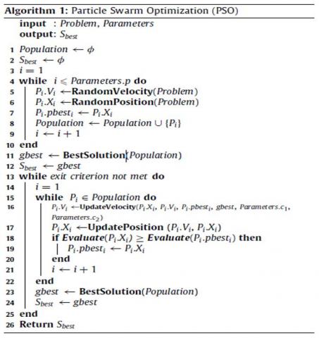
PSO is a population-based algorithm that mimics the social behaviors of flocks of birds and fish swarms. This algorithm was first introduced by Kennedy and Eberhart [25]. PSO is beneficial for performing feature selection because of its ease of implementation, speed of convergence and low compute cost [26, 27]. In the PSO algorithm [25, 28], a swarm consists of a set of particles (Population). Each particle "i" represents a candidate solution and has the speed "vi" and position "xi". The problem is optimized by improving each candidate solution by the motion of the corresponding particle in the research space. The motion of a particle is influenced by the best local position "pbest" of the particle as well as the best overall solution for the swarm "gbest", which corresponds to the particle with the best pbest. The evaluation of pbest and gbest depends on an objective function (fitness function), which measures the degree of effectiveness of the solution of each particle. During motion, each particle in the swarm updates its "vi" speed and "xi" position using:
$v_i(t+1)=w * v_i(t)+c_1 * r_1\left(\right.$ pbest $\left._i-x_i(t)\right)+c_2 * r_2\left(\right.$ gbest $\left.-x_i(t)\right)$ (43)
$x_i(t+1)=x_i(t)+v_i(t+1)$ (44)
where, vi(t+1) represents the new speed of the particle, c1 and c2 are the acceleration coefficients, w is an inertial weight, r1 and r2 are random numbers, vi(t) is the velocity of particle i at time t, xi(t) is the velocity of particle i at time t, pbesti is the best position occupied by particle i at time t, gbest is the best position discovered by the swarm at time t, and xi(t+1) is the new position of the particle.
Algorithm 1 presents the pseudocode of the PSO algorithm, where Random Position and Random Velocity are used to initialize each particle with a random initial position and a random initial velocity, respectively; Best solution returns the best solution among all the particles in the swarm; Update Velocity returns the new velocity value of a particle using Eq. (43); Updating Position returns the new position of a particle using Eq. (44), and calculates the fitness value of a solution.
In the abovementioned explanation of the PSO algorithm, a continuous space is assumed; however, in this article, we use a version of PSO known as BPSO [29], which was developed to solve discrete problems. In addition, BPSO is one of the most effective methods of selecting packaging characteristics [26, 27]. In BPSO, the speed vi represents the probability that xi will take a value of 1 or 0. To restrict all real position values to 0 or 1, the sigmoid function is applied using:
$x_i= \begin{cases}1 \quad \text { if } \operatorname{rand}(0,1)<S\left(v_i\right)\\ 0 \quad \text {else}\end{cases}$ (45)
$S\left(v_i\right)=\frac{1}{1+e^{-v_i}}$ (46)
where, rand (xi) is a random uniform number in the interval [0, 1]. The updated position is normalized using S(vi), where $v_i$ denotes the updated speed of the particle. When S(vi) is greater than the random number generated, the position value of the particle (xi) is 1; otherwise, xi is 0.
The BPSO parameters and the problem of interest, which consist of the feature set, are passed to the PSO algorithm (Algorithm 1). The velocities and positions of the particles are updated according to Eq. (43) and Eq. (45), respectively. The main objective of this study is to improve the performance of the classifier. The Evaluate evaluation function is defined based on the accuracy results of the classifier, and the output is determined as Evaluate (y)=Accuracy (y). Precision (y) refers to the accuracy of the classifier for the model formed and tested using the subset of characteristics selected there by the particle evaluated in the PSO swarm. Subsequently, the Best Solution function returns the solution (a subset of characteristics (y)) with the best accuracy value obtained among the population.
4.3 Principal component analysis algorithm (PCA)
Suppose that observations for m features form an n×m matrix, signe as X=(xij) i=1, 2, .., n, j= 1, 2…, m. The PCA is processed as follows [30].
·Standardize the data as (47):
$x_{i j}=\frac{x_{i j}-x_{j, \text { mean }}}{\sigma\left(x_j\right)}$ (47)
·Calculate m*m correlation matrix C as (48), which is symmetrical and positive definite:
$C=X^T X$ (48)
·The eigenvalue λi and the eigenvector Pj of C is calculated in descending order of magnitude (λ1>λ2>…>λm). The original data can then be expressed in terms of eigenvalues and eigenvectors, which define the directions of the principal components as (49):
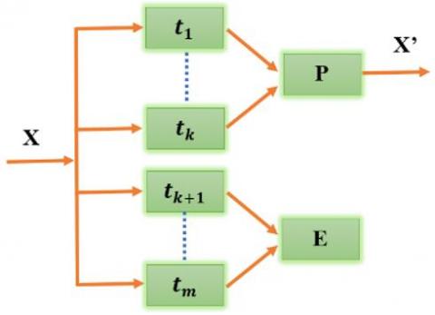
$X=t_1 p_1^T+t_2 p_2^T+\cdots+t_k p_k^T+E$ (49)
where, $E=t_{k+1} p_{k+1}^T+t_{k+2} p_{k+2}^T+\cdots+t_m p_m^T$. Eq. 49 can be rewritten in matrix form as (50):
$X=T P^T+E$ (50)
where, T=[t1, t2, …, tk] with k<m is called the principal component score, P=[p1, p2, …, pk] is called the principal component loads. E is the residue and k(k<m) is the number of scores. The condition of optimization Eq. (50) is that the Euclidean norm of the residual matrix E must be minimized. To satisfy this criterion, it was shown that P=[p1, p2, …, pk] is the eigenvector of the covariance matrix of X.
An approximate model, including the first k terms of Eq. 49, will capture most of the observed variance X if the data are correlated. The percentage by which the information in X can be expressed as the first k terms of the principals is Q, which can be expressed as Eq. (51):
$Q=\frac{\lambda_1+\lambda_2+\cdots+\lambda_K}{\sum_{j=1}^m \lambda_j}$ (51)
From Eq. (47) and Eq. (48), scores can be obtained in Eq. (52):
T=XP (52)
The PCA is a linear mapping of the original observed data. The load vector P is the linear transformation coefficient. After obtaining P and T, the reconstructed data can be written as Eq. (53):
$X^{\prime}=T P^T+E$ (53)
where, X'=[x1, x2, …, xk]T is the reconstruction of the observed data and the dimensions of the data are reduced from m to k(k<m), the principle of PCA is illustrated in Figure 14. The method of determining the number (k) of the principal components is the key to the application of the PCA [30].
Figure 14. The principle of PCA
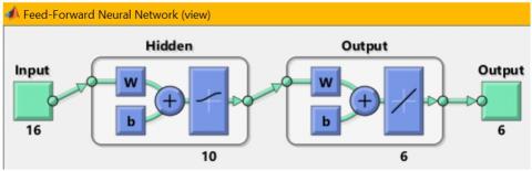
In this work, a feed-forward neural network (ANN) is applied with a hidden layer of 10 neurons (Figure 15) and a random forest (RF) with 20 trees to perform the four training and testing cases (without optimization and with BBAT, BPSO, PCA optimization algorithms). The results obtained are shown in Table 4. But the best results of hybrid parameters (statistical and wavelet packet decomposition) with PCA are inserted in part (6).
The first step is to acquire samples of Ias current from healthy motors and fault motors with rotor broken bars. This current data is used as input into the signal processing stage. The healthy and faulty motor current samples used in this study were obtained from the simulation results of the multi-wind model of the broken rotor bars.
The size of the input data set used is 600-by-17 matrix and target output data is 600-by-6 matrix whose outputs are binary in nature where a vector output of [1; 0; 0; 0; 0; 0] healthy motor condition, [0; 1; 0; 0; 0; 0] presence of one broken rotor bar until [0; 0; 0; 0; 0; 1] presence of Three distant rotor broken bars (Table 3). 70% of the data set is used for ANN training and the rest for testing.
Table 3. Classification of several faults
|
Fault type |
Symbol |
Code |
|||||
|
|
S1 |
S2 |
S3 |
S4 |
S5 |
S6 |
|
|
Healthy state |
HS |
1 |
0 |
0 |
0 |
0 |
0 |
|
One broken rotor bar |
OBRB |
0 |
1 |
0 |
0 |
0 |
0 |
|
Two adjacent rotor broken bars |
TARBB |
0 |
0 |
1 |
0 |
0 |
0 |
|
Two distant rotor broken bars |
TDRBB |
0 |
0 |
0 |
1 |
0 |
0 |
|
Three adjacent rotor broken bars |
THARBB |
0 |
0 |
0 |
0 |
1 |
0 |
|
Three distant rotor broken bars |
THDRBB |
0 |
0 |
0 |
0 |
0 |
1 |
Initially, all statistical and wavelet packet features were evaluated without performing feature screening; the results are shown in Table 4. ANN and RF using hybrid features (statistical and wavelet packet parameters) for detection of healthy and broken rotor bar faults states produced higher accuracy than the other combinations. The RF classifier with PCA achieved the highest accuracy (98.333%) among all classifiers with different types of characteristics.
Table 4. Results of ANN and RF classifiers without and with optimization algorithms
|
|
Statistical parameters |
Wavelet Packet Decomposition parameters |
Hybrid (statistical and Wavelet Packet Decomposition) parameters |
||||||||||
|
Training |
Testing |
Training |
Testing |
Training |
Testing |
||||||||
|
ANN |
RF |
ANN |
RF |
ANN |
RF |
ANN |
RF |
ANN |
RF |
ANN |
RF |
||
|
Without optimization |
Accuracy % |
81.1905 |
100 |
76.1111 |
87.2222 |
86.1905 |
98.8095 |
78.8889 |
79.4444 |
95.4762 |
100 |
87.7778 |
90 |
|
Time (s) |
109.8219 |
13.5052 |
2.7616 |
8.1943 |
63.207 |
12.0571 |
2.6618 |
4.9598 |
127.3953 |
12.0414 |
6.3246 |
4.6141 |
|
|
BBAT |
Accuracy % |
78.3333 |
99.7619 |
75.5556 |
87.2222 |
85.4762 |
99.2857 |
81.1111 |
78.3333 |
90.9524 |
99.7619 |
91.1111 |
92.7778 |
|
Time (s) |
41.2341 |
11.5924 |
2.5658 |
4.7801 |
54.2727 |
11.9094 |
2.5868 |
5.1606 |
55.3485 |
11.5786 |
2.556 |
4.7123 |
|
|
BPSO |
Accuracy % |
84.0476 |
99.7619 |
83.8889 |
88.3333 |
82.8571 |
99.7619 |
78.3333 |
78.8889 |
94.7619 |
99.7619 |
93.8889 |
95 |
|
Time (s) |
50.7143 |
11.8571 |
2.5342 |
4.9335 |
46.0295 |
11.8125 |
2.6083 |
4.8937 |
88.9211 |
11.6481 |
2.5552 |
4.8687 |
|
|
PCA |
Accuracy % |
75.4762 |
99.7619 |
81.1111 |
89.4444 |
93.8095 |
100 |
93.8889 |
96.1111 |
98.0952 |
100 |
97.2222 |
98.3333 |
|
Time (s) |
63.5083 |
12.2038 |
2.7196 |
4.9923 |
103.6447 |
13.513 |
3.8241 |
6.1582 |
77.4085 |
11.7981 |
2.8647 |
4.8404 |
|
6.1 Classification using a hybrid parameter with PCA
·Classification using artificial neural network
Figure 15. Feed-forward neural network with PCA
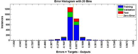
Figure 16. Error histogram between target values and predicted values of ANN with PCA
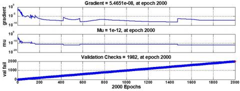
Figure 17. Training state of ANN with PCA
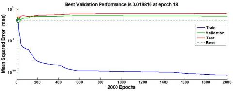
Figure 18. Mean square error of 2000 Epochs for the ANN with PCA
·Classification using Random Forest
Figure 19. The balanced error rate of RF with PCA
A histogram of an error after training ANN and Training state. with PCA optimization algorithm is shown in Figure 16, 17. Moreover, validation performance is shown in Figure 18. The mean squared error of 2000 epochs shows the best validation performance at epoch 18.
Several tests of classification using random forest -by increasing the number of trees- have been done. From the result illustrated in Figure 19. we can conclude that the balanced error rate of RF decreases when the number of trees increases. It can be seen also that the best-balanced error rate is obtained using 20 trees, for this reason the value (0.1142) it will be considered as the best random forest classifier.
Classification of the healthy and defective state of the rotor bars of the induction machine with artificial intelligence techniques like ANN and Random Forest assisted by the algorithms of features selection like BBAT, BPSO, and features reduction like PCA from the statistical parameters and wavelet packet decomposition parameters are all shown on both Tables 4 and 5.
Table 5. Optimized dimensionality reduction algorithm for fault diagnosis of rotor broken bars in induction machine
|
Features |
Original inputs without optimization algorithms |
Reduction inputs with optimization algorithms |
||
|
BBAT |
BPSO |
PCA |
||
|
Statistical |
9 |
4 |
4 |
8 |
|
wavelet packet decomposition |
8 |
4 |
5 |
7 |
|
Hybrid (statistical and wavelet packet decomposition) |
17 |
6 |
7 |
16 |
The detection and early diagnosis allow for reducing damage and maintaining other components of induction machine, through the study of defects influence and the behavior of the machine in case of operation fault. In this paper, we presented the induction machine fault by using a multi-winding model for the simulation of broken bars. The proposed diagnosis method could be applied by artificial intelligence represented by neural networks (ANN) and random forest (decision tree) with BBAT, BPSO, and PCA optimization algorithms on induction machine during several parametric studies (selection of the type of network, choice of inputs, and choice of outputs, number of trees in the random forest, ...). The data acquisition operation, to establish the learning machine base. To be reliable indicators for detection and location of fault broken bars. These results indicate clearly that the proposed RF with optimization algorithm PCA used hybrid parameters (statistical and wavelet packet decomposition parameters) and followed by PCA gave high accuracy (98.3333%), it has great importance for fault identification, and it is capable to reduce the failure severity. Furthermore, it has been manifested that this approach is accurate and simple in the process implement diagnosis.
[1] Bhasme, D.A., Chavhan, V.S. (2020). Induction motor condition monitoring system based on machine learning. International Research Journal of Engineering and Technology (IRJET), 7(5): 6590-6593.
[2] Chouidira, I., Eddine, K.D., Benguesmia, H. (2019). Detection and diagnosis faults in machine asynchronous based on single processing. International Journal of Energetica (IJECA), 4(1): 11-16. http://dx.doi.org/10.47238/ijeca.v4i1.89
[3] Sadeghian, A., Ye, Z., Wu, B. (2009). Online detection of broken rotor bars in induction motors by wavelet packet decomposition and artificial neural networks. IEEE Transactions on Instrumentation and Measurement, 58(7): 2253-2263. https://doi.org/10.1109/TIM.2009.2013743
[4] Garcia-Calva, T.A., Morinigo-Sotelo, D., Fernandez-Cavero, V., Garcia-Perez, A., Romero-Troncoso, R.D.J. (2021). Early detection of broken rotor bars in inverter-fed induction motors using speed analysis of startup transients. Energies, 14(5): 1469. https://doi.org/10.3390/en14051469
[5] Gangsar, P., Tiwari, R. (2019). A support vector machine based fault diagnostics of Induction motors for practical situation of multi-sensor limited data case. Measurement, 135: 694-711. https://doi.org/10.1016/j.measurement.2018.12.011
[6] Aerhpanahi, M., Sadeghi, S.H.H., Roknabadi, H.A. (2004). Broken rotor bar detection in induction motor via stator current derivative. In 2004 IEEE International Conference on Industrial Technology, 2004. IEEE ICIT'04, pp. 1363-1367. https://doi.org/10.1109/ICIT.2004.1490759
[7] Laala, W., Zouzou, S.E., Guedidi, S. (2014). Induction motor broken rotor bars detection using fuzzy logic: experimental research. International Journal of System Assurance Engineering and Management, 5(3): 329-336. https://doi.org/10.1007/s13198-013-0171-8
[8] Supangat, R., Ertugrul, N., Soong, W.L., Gray, D.A., Hansen, C., Grieger, J. (2006). Detection of broken rotor bars in induction motor using starting-current analysis and effects of loading. IEE Proceedings-Electric Power Applications, 153(6): 848-855. http://dx.doi.org/10.1049/ip-epa:20060060
[9] Menacer, A., Nait-Said A, M.S., Benakcha, H., Drid, S. (2004). Stator current analysis of incipient fault into asynchronous motor rotor bars using Fourier fast transform. Journal of Electrical Engineering-Bratislava, 55: 122-130.
[10] Allal, A., Khechekhouche, A. (2022). Diagnosis of induction motor faults using the motor current normalized residual harmonic analysis method. International Journal of Electrical Power & Energy Systems, 141: 108219. https://doi.org/10.1016/j.ijepes.2022.108219
[11] Chen, S., Živanović, R. (2010). Modelling and simulation of stator and rotor fault conditions in induction machines for testing fault diagnostic techniques. European Transactions on Electrical Power, 20(5): 611-629. https://doi.org/10.1002/etep.342
[12] Sabir, H., Ouassaid, M., Ngote, N. (2022). An experimental method for diagnostic of incipient broken rotor bar fault in induction machines. Heliyon, e09136. https://doi.org/10.1016/j.heliyon.2022.e09136
[13] Chouidira, I., Khodja, D., Chakroune, S. (2019). Induction machine faults detection and localization by neural networks methods. Rev. d'Intelligence Artif., 33(6): 427-434. https://doi.org/10.18280/ria.330604
[14] Khodja, D.E., Kheldoun, A. (2009). Three-phases model of the induction machine taking account the stator faults. World Academy of Science, Engineering and Technology, 3(4): 363-366.
[15] Trajin, B. (2008). Détection automatique et diagnostic des défauts de roulements dans une machine asynchrone par analyse spectrale des courants statoriques. Conférences des jeunes chercheurs en Génie électrique, 16-17 December 2008 (Lyon, France).
[16] Baghli, L. (1999). Contribution à la commande de la machine asynchrone, utilisation de la logique floue, des réseaux de neurones et des algorithmes génétiques (Doctoral dissertation, Université Henri Poincaré-Nancy I).
[17] Roland, U., Eseosa, O. (2014). Artificial intelligent techniques in real-time diagnosis of stator and rotor faults in induction machines. Int. J. Sci. Eng. Res, 5(10): 946-954.
[18] Ye, Z., Wu, B., Sadeghian, A. (2003). Current signature analysis of induction motor mechanical faults by wavelet packet decomposition. IEEE Transactions on Industrial Electronics, 50(6): 1217-1228. https://doi.org/10.1109/TIE.2003.819682
[19] Sarkar, T.K., Salazar-Palma, M., Wicks, M.C. (2002). Wavelet applications in engineering electromagnetics. Artech House.
[20] Tarasiuk, T. (2004). Hybrid wavelet-Fourier spectrum analysis. IEEE Transactions on Power Delivery, 19(3): 957-964. https://doi.org/10.1109/TPWRD.2004.824398
[21] Rajagopalan, S., Aller, J.M., Restrepo, J.A., Habetler, T.G., Harley, R.G. (2007). Analytic-wavelet-ridge-based detection of dynamic eccentricity in brushless direct current (BLDC) motors functioning under dynamic operating conditions. IEEE Transactions on Industrial Electronics, 54(3): 1410-1419. https://doi.org/10.1109/TIE.2007.894699
[22] Mirjalili, S., Mirjalili, S.M., Yang, X.S. (2014). Binary bat algorithm. Neural Computing and Applications, 25(3): 663-681. https://doi.org/10.1007/s00521-013-1525-5
[23] Li, G., Le, C. (2019). Hybrid binary bat algorithm with cross-entropy method for feature selection. In 2019 4th International Conference on Control and Robotics Engineering (ICCRE), pp. 165-169. https://doi.org/10.1109/ICCRE.2019.8724270
[24] Mirjalili, S., Hashim, S.Z.M. (2012). BMOA: binary magnetic optimization algorithm. International Journal of Machine Learning and Computing, 2(3): 204. https://doi.org/10.7763/IJMLC.2012.V2.114
[25] Kennedy, J., Eberhart, R. (1995). Particle swarm optimization. In Proceedings of ICNN'95-international conference on neural networks, pp. 1942-1948. https://doi.org/10.1109/ICNN.1995.488968
[26] Brezočnik, L., Fister Jr, I., Podgorelec, V. (2018). Swarm intelligence algorithms for feature selection: A review. Applied Sciences, 8(9): 1521. https://doi.org/10.3390/app8091521
[27] Nguyen, B.H., Xue, B., Zhang, M. (2020). A survey on swarm intelligence approaches to feature selection in data mining. Swarm and Evolutionary Computation, 54: 100663. https://doi.org/10.1016/j.swevo.2020.100663
[28] Eberhart, R.C., Shi, Y., Kennedy, J. (2001). Swarm intelligence. Elsevier. Book ISBN: 9780080518268. Hardcover ISBN: 9781558605954
[29] Kennedy, J., Eberhart, R.C. (1997). A discrete binary version of the particle swarm algorithm. In 1997 IEEE International Conference on Systems, Man, and Cybernetics. Computational Cybernetics and Simulation, pp. 4104-4108. https://doi.org/10.1109/ICSMC.1997.637339
[30] Yu, C.Q., Guo, X.S., Zhang, A., Pan, X.J. (2007). An improvement algorithm of principal component analysis. In 2007 8th International Conference on Electronic Measurement and Instruments. http://dx.doi.org/10.1109/ICEMI.2007.4350734