Riad Benghalia* | Ahmed Cheriet | Ishaq Amrani
© 2020 IIETA. This article is published by IIETA and is licensed under the CC BY 4.0 license (http://creativecommons.org/licenses/by/4.0/).
OPEN ACCESS
Currently, many simulation tools based on numerical methods are available for modelling of low frequency electromagnetic problems such as eddy current related problems, electrical machines and electromagnetic actuators analysis. Commonly, it’s the finite element method (FEM) which is used; nevertheless, the exploit of other numerical approaches, such as the finite volume method (FVM) can be strongly promising. Accordingly, the main purpose of this paper is to present the FVM method as an alternative method for low frequency electromagnetic problems. Thus, 2D and 3D FVM computer codes are developed and examined through the analysis of two TEAM workshop problems and an experimental electromagnetic micro-actuator. These types of problems are habitually analyzed by the FEM method. By using the FVM method, the solution of the above listed problems includes eddy current, torque and magnetic force computation.
3D triangular mesh, FVM, force, torque, dynamics
Computational electromagnetic tools are impressively indispensable for analysing and optimization of electromagnetic devices such as electrical machines. These numerical tools help powerfully designers in order to minimize both time and cost. At the present time, many simulation tools based on numerous numerical methods are commercially available even for low (LF) or high (HF) frequency electromagnetic problems. For LF electromagnetic problems such as related to eddy current analysis or magnetic force computation, it is the finite element method (FEM) which is commonly used according to its efficiency. What's more, because the method is enough developed and famously known throughout the scientific community in electromagnetic. However, there exist other numerical methods which can be as well extremely promising for LF electromagnetic problems, such as the finite volume method (FVM). Several previous works have been interested in the comparison between the FVM and the FEM regarding various physical problems [1-4]. Compared to the FEM, the FVM method is especially promising in terms of computational time (CPU) and required storage memory [5-7]. Originally, the FVM method is applied for the solution of problems related to fluid flows [8, 9]. Then, the FVM method is applied to solve Maxwell's equations in the HF domain such as in wave propagation problems [10, 11]. The method is applied moreover to solve some electrostatic problems such as in the study [12]. In the last few years, the FVM is presented as a new method to solve LF electromagnetic problems [13, 14] where quasi-static magnetic field is analysed. As well, other researchers are interesting in developing FVM in time domain to analyze nonlinear electromagnetic field [15].
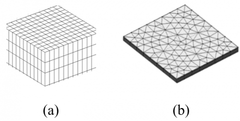
For 3D LF electromagnetic problems, note that the FVM method has been already developed where a simple hexahedral volume element is used [16, 17] (Figure 1.a). Thus, in order to handle more complex geometries, this paper proposes a 3D unstructured FVM by making use of prism element (Figure 1.b).
Figure 1. Control volume shape for 3D FVM method
(a) Hexahedral mesh, (b) Prism mesh
As well, for 2D LF electromagnetic problems, a simple rectangular control volume is usually associated to the FVM [18]. Furthermore, to give more flexibility to the FVM to analyze more complex geometries in the 2D case, this paper proposes in addition a 2D unstructured FVM by making use of triangular mesh.
To check the developed computing codes, two TEAM workshop problems and an experimental electromagnetic micro-actuator are analyzed. The solution of 1st TEAM includes the determination of levitation height of an aluminium plate and the applied magnetic force, while the 2nd one requires torque computation. The two TEAM problems require eddy current computation for either force or torque computation. The third problem is related to magnetic force computation and dynamic analyses.
To give an idea as well as more details on the FVM method, in this section we will study the FVM in both cases 2D with triangular element and 3D with prism volume. For both cases, starting from Maxwell’s equations [19], in terms of the magnetic vector potential A, the equation to solve is:
$\nabla \times \frac{1}{\mu} \nabla \times \mathbf{A}=\mathbf{J}_{\mathrm{s}}+\mathbf{J}_{i n d}$ (1)
$\mathbf{A}=0$ at infinity (2)
μ is the magnetic permeability, Js is the source current density and Jind is the eddy current density. Eq. (2) describes the impressed Dirichlet condition at infinity.
2.1 2D case
In the 2D case the magnetic flux density is defined only in the Oxy plan and consequently the magnetic vector potential and the source current density have only one component as:
$\mathbf{A}=A_{z} \mathbf{k}$ (3)
$\mathbf{J}_{s}=J_{s z} \mathbf{k}$ (4)
where, k is the unit vector in the z direction. Thus, in this case Eq. (1) can be rewritten as:
$-\nabla \cdot\left(\frac{1}{\mu} \nabla A_{z}\right)=J_{s z} \mathbf{k}+\mathbf{J}_{i n d}$ (5)
The eddy current density, which is induced either by movement or temporal variation of the current source, is given by:
$\mathbf{J}_{\text {ind}}=\sigma\left(-\frac{\partial A_{z}}{\partial t} \mathbf{k}+\mathbf{v} \times \mathbf{B}\right)$ (6)
In Eq. (6) v is the velocity, B is the magnetic flux density and $\sigma$ is the electrical conductivity. In the 2D case; the velocity term can be rewritten as follows:
$\mathbf{v} \times \mathbf{B}=-\left(v_{x} \cdot \frac{\partial A_{z}}{\partial x}+v_{y} \cdot \frac{\partial A_{z}}{\partial y}\right) \mathbf{k}$ (7)
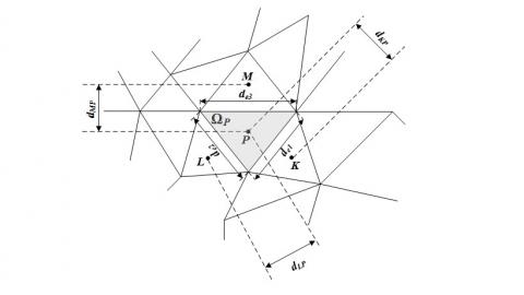
Figure 2. Triangular mesh scheme for 2D FVM method
vx and vy are the velocity components in the Oxy plan. By substituting Eq. (7) in Eq. (6), and by using the harmonic representation, Eq. (5) becomes:
$-\nabla \cdot\left(\frac{1}{\mu} \nabla A_{z}\right)+\sigma\left(j \omega A_{z}+v_{x} \cdot \frac{\partial A_{z}}{\partial x}+v_{y} \cdot \frac{\partial A_{z}}{\partial y}\right) \mathbf{k}=J_{s z} \mathbf{k}$ (8)
At this stage, Eq. (8) has to be solved by the 2D FVM method with triangular mesh. As described in Figure 2, in the case of triangular mesh scheme, each principal control volume Ωp is represented by its principal node P and surrounded by three neighbourhood control volumes represented by their nodes K, L and M.
Subsequently, the FVM method involves a surface integration of Eq. (8) over the principal control volume Ωp of node P as:
$\iint_{\Omega_{p}}-\nabla \cdot\left(\frac{1}{\mu} \nabla A_{z}\right) \mathrm{d} \Omega+\iint_{\Omega_{p}} \sigma \omega A_{z} \mathrm{jd} \Omega$
$+\iint_{\Omega_{p}} \sigma\left(v_{x} \cdot \frac{\partial A_{z}}{\partial x}+v_{y} \cdot \frac{\partial A_{z}}{\partial y}\right) \mathrm{d} \Omega=\iint_{\Omega_{p}} J_{s z} \mathrm{d} \Omega$ (9)
The first term in Eq. (9) can be rewritten as follows:
$\begin{align} & \iint\limits_{{{\Omega }_{p}}}{-\nabla .\left( \frac{1}{\mu }\nabla {{A}_{z}} \right)}d\Omega =-\frac{1}{\mu }\oint\limits_{\partial {{\Omega }_{p}}}{\nabla {{A}_{z}}.\mathbf{n}.\mathbf{dl}} \\ & \begin{matrix} \begin{matrix} \begin{matrix} {} & {} \\\end{matrix} & {} \\\end{matrix} & {} & {} & {} \\\end{matrix}=-\frac{1}{\mu }\sum\limits_{i=1}^{3}{\nabla {{A}_{z}}.{{\mathbf{n}}_{i}}.{{d}_{ei}}} \\\end{align}$ (10)
n is the normal vector and dei is the ith edge length with respect to i=1, 2, 3. The term $\nabla A_{z} \cdot \boldsymbol{n}_{i}$ can be approximated for each edge by a finite difference, for example for the edge de1:
$\left(\nabla A_{z} \cdot \mathbf{n}_{1}\right)_{d e 1}=\frac{A_{z}^{K}-A_{z}^{P}}{d_{K P}}$ (11)
By the way, Eq. (10) leads to an algebraic expression as:
$-\frac{1}{\mu} \sum_{i=1}^{3} \nabla A_{z} \mathbf{n}_{i} \cdot d_{e i}=-\frac{1}{\mu}\left[\frac{A_{z}^{K}-A_{z}^{P}}{d_{K P}} \cdot d_{e 1}\right.$$\left.+\frac{A_{z}^{L}-A_{z}^{P}}{d_{L P}} \cdot d_{e 2}+\frac{A_{z}^{M}-A_{z}^{P}}{d_{M P}} \cdot d_{e 3}\right]$ (12)
Eq. (12) can be rewritten as follows:
$-\frac{1}{\mu} \sum_{i=1}^{3} \nabla A_{z} \mathbf{n}_{i} \cdot d_{e i}=\frac{1}{\mu}\left(\frac{d_{e 1}}{d_{K P}}+\frac{d_{e 2}}{d_{L P}}+\frac{d_{e 3}}{d_{M P}}\right) \cdot A_{z}^{P}$$-\frac{1}{\mu}\left(\frac{d_{e 1}}{d_{K P}} \cdot A_{z}^{K}+\frac{d_{e 2}}{d_{L P}} \cdot A_{z}^{L}+\frac{d_{e 3}}{d_{M P}} \cdot A_{z}^{M}\right)$ (13)
Let’s assume a uniform distribution of the current density in the principal control volume Ωp. Therefore, the source term is integrated as follows:
$\iint_{\Omega p} J_{sz} d \Omega=J_{szP} \cdot S_{\Omega p}$ (14)
The integration of all terms given by Eq. (9) leads in an algebraic equation that express the potential in the principal control volume in terms of potentials of its three neighbourhoods as:
$A_{z}^{P}=\frac{1}{C_{p}}\left(C_{\mathrm{k}} A_{z}^{K}+C_{1} A_{z}^{L}+C_{\mathrm{m}} A_{z}^{M}+J_{\mathrm{szP}} S_{\Omega p}\right)$ (15)
The coefficients Cp, Ck, Cl and Cm describe geometrical and physical properties associated with the principal control volume and its neighbourhoods. JszP is the current density in the principal control volume. Rewriting Eq. (15) for all control volumes, thus leads to the following matrix equation:
$\left[\mathbf{M}_{2}\right]\left[A_{z}\right]=\left[J_{s z}\right]$ (16)
Compared to the FEM method, we point out that the FVM method leads to a sparser matrix M2; this particular property are very significant regards to computational time and required storage memory.
2.2 3D case
The 3D standard FVM method featured by hexahedral control volume shape has been already demonstrated in previous works showing its effectiveness for electromagnetic devices. Unfortunately, the hexahedral element appears too cost in the case of complex geometry, such as for example for circular coils. To overcome the limitation of the standard FVM method and enable it to handle more complex geometry, we propose a 3D unstructured FVM method. In such alternative the simple hexahedral control volume is replaced by a prism control volume (Figure 3).
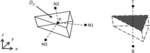
Figure 3. Prism control volume for 3D FVM method
Here, each control volume element Dp consists of a central node P and delimited by five faces. The neighbourhood control volumes of Dp are represented by their central nodes K, L and M in the Oxy plan, B and T according to the z direction. As in the 2D case, Eq. (1) must be integrated over the prism control volume:
$\int_{z}\left[\iint_{\Omega_{p}}\left(\nabla \times \frac{1}{\mu} \nabla \times \mathbf{A}\right) d \Omega_{p}\right] d z=\int_{z}\left[\iint_{\Omega_{p}}\left(\mathbf{J}_{\mathrm{s}}+\mathbf{J}_{i n d}\right) d \Omega_{p}\right] d z$ (17)
with:
$d \Omega_{p} d z=d D_{p}$ (18)
According to the Green-Ostrogradsky theorem, Eq. (17) becomes:
$-\iiint_{D_{p}}\left(\nabla \cdot\left(\frac{1}{\mu} \nabla \mathbf{A}\right)\right) \mathrm{d} D_{p}=\iiint_{D_{p}}\left(\mathbf{J}_{\mathrm{s}}+\mathbf{J}_{i n d}\right) \mathrm{d} D_{p}$ (19)
For the first term we have:
$-\iiint\limits_{Dp}{\nabla .(\frac{1}{\mu }\nabla A)d}{{D}_{p}}=-\mathop{{\int\!\!\!\!\!\int}\mkern-21mu \bigcirc}\limits_S \frac{1}{\mu } \nabla A.d\mathbf{s}$ (20)
Let consider for example the integration of the x component:
$-\mathop{{\int\!\!\!\!\!\int}\mkern-21mu \bigcirc}\limits_s \frac{1}{\mu } \nabla {{A}_{x}}.ds.\mathbf{n}=-\sum\limits_{i=1}^{5}{\frac{1}{{{\mu }_{i}}}\nabla {{A}_{x}}.d{{\mathbf{s}}_{i}}}$
$=-\left[\frac{S_{1}}{\mu_{1}} \frac{A_{x 1}-A_{x p}}{d l_{1} \sin \left(d e_{1}, d l_{1}\right)}+\frac{S_{2}}{\mu_{2}} \frac{A_{x 2}-A_{x p}}{d l_{2} \sin \left(d e_{2}, d l_{2}\right)}\right.$
$+\frac{S_{3}}{\mu_{3}} \frac{A_{x 3}-A_{x p}}{d l_{3} \sin \left(d e_{3}, d l_{3}\right)}+\frac{S_{4}}{\mu_{4}} \frac{A_{x 4}-A_{x p}}{d l_{4} \sin \left(d e_{4}, d l_{4}\right)}$
$\left.+\frac{S_{5}}{\mu_{5}} \frac{A_{x 5}-A_{x p}}{d l_{5} \sin \left(d e_{5}, d l_{5}\right)}\right]$ (21)
Let us define the first coefficient as:
$C_{1}=\frac{S_{1}}{\mu_{1}} \frac{1}{d l_{1} \sin \left(d e_{1}, d l_{1}\right)}$ (22)
Subsequently, all the coefficients in the previous algebraic equation can be rewritten as the the following general form:
$C_{i}=\frac{S_{i}}{\mu_{i}} \frac{1}{d l_{i} \sin \left(d e_{i}, d l_{i}\right)}$ (23)
The developpement of the x component of the first term leads to the following algebraic equation:
$-\left(C_{1}\left(A_{x 1}-A_{x p}\right)+C_{2}\left(A_{x 2}-A_{x p}\right)+C_{3}\left(A_{x 3}-A_{x p}\right)\right.$
$\left.+C_{4}\left(A_{x 4}-A_{x p}\right)+C_{5}\left(A_{x 5}-A_{x p}\right)\right)=\left[-\left(C_{1} A_{x 1}+C_{2} A_{x 2}\right.\right.$
$\left.+C_{3} A_{x 3}+C_{4} A_{x 4}+C_{5} A_{x 5}\right)$
$\left.+A_{x p}\left(C_{1}+C_{2}+C_{3}+C_{4}+C_{5}\right)\right]$ (24)
By assuming that the current density is constant within the control volume, the x component of the potential in the central node P is given by:
$A_{x p}=\frac{1}{C_{p}}\left(\sum_{i=1}^{5} C_{i} A_{x i}-C_{6} \frac{V_{x 2}-V_{x 1}}{d x}+C_{x s}\right)$ (25)
Cp, C1, C2, C3, C4, C5and C6, describe geometrical and physical properties associated with the principal control volume and its five neighbourhoods. Vxi is the electrical potential. Similarly, we can find both y and z components of the potential in the central node as:
$A_{y p}=\frac{1}{C_{p}}\left(\sum_{i=1}^{5} C_{i} A_{y i}-C_{6} \frac{V_{y 2}-V_{y 1}}{d y}+C_{y s}\right)$ (26)
$A_{z p}=\frac{1}{C_{p}}\left(\sum_{i=1}^{5} C_{i} A_{z i}-C_{6} \frac{V_{z 2}-V_{z 1}}{d z}+C_{z s}\right)$ (27)
These last three equations can be rewritten in a matrix form as:
$\left[\mathbf{M}_{3}\right][\mathbf{A}]=\left[\mathbf{J}_{s}\right]$ (28)
As in the 2D case, the 3D FVM method leads to sparse and symmetric matrix M3; this feature is strongly significant regards to computational time and required storage memory especially for the 3D case. By the way, both 2D and 3D computer codes are developed in Matlab. To check the developed computer codes, two TEAM workshop problems and an experimental electromagnetic micro-actuator are analyzed in the next sections.
3.1 TEAM workshop problem No. 30
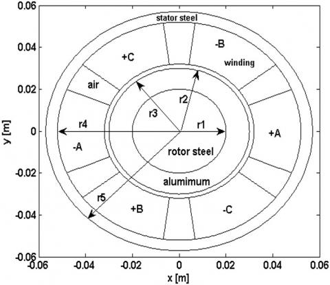
The TEAM Workshop problem No.30 deals with a special three phase induction motor, in which the eddy current in the rotor is induced by the time harmonic current in the stator windings, and by the rotation of the rotor [20]. The arrangement of the three phase coils A, B and C is shown in Figure 4. The rotor angular velocity is ranging from 0 to 1200 rad/s. In this special three phase induction motor, the windings are not embedded in slots and the rotor is made of steel and aluminium with depth of 100cm. The relative magnetic permeability of the steel is μr = 30. The motor is supplied with current density 310A/cm2, 60Hz.
Figure 4. Description of TEAM workshop problem No. 30 r1=2, r2=3, r3=3.2, r4=5.2, r5=5.7, cm
To solve this problem, the developed 2D FVM computer code using triangular mesh is used. Thus, both fundamental quantities of the motor are computed i.e. the electromagnetic torque and the induced voltage in the phase coil A. The electromagnetic torque is calculated by using the following equation:
$C_{e m}=\mathbf{r} \times d V \times \mathbf{J}_{i n dz} \times \mathbf{B}$ (29)
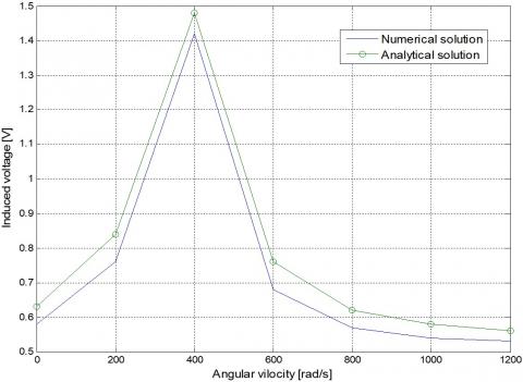
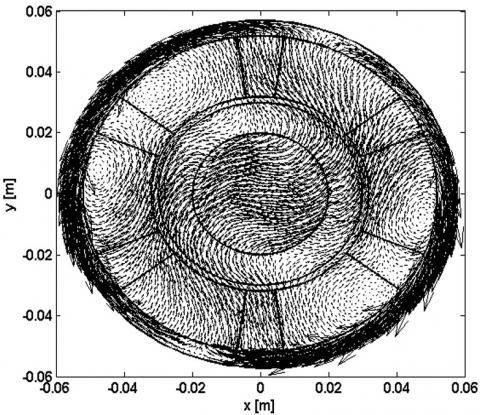
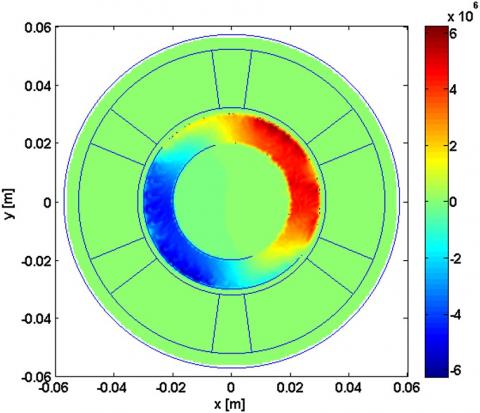
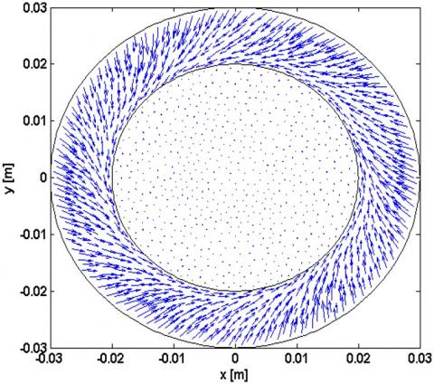
Table 1, Figure 5 and Figure 6, illustrate a comparison of the fundamental quantities of the motor, in which we recognize a very small difference between the 2D FVM solution and the analytical solution provided by the TEAM workshop problem. Both results appear to be comparable at all angular velocity of the rotor. Figure 7, Figure 8 and Figure 9 show respectively, the magnetic flux density vectors, the induced current density in the rotor and the electromagnetic force vectors in the rotor at angular velocity of 200 rad/s. As expected, this modelling makes obvious that the finite volume method is a competitive method in the solution of problems related to eddy current and electromagnetic torque computation in the 2D case.
Figure 5. The electromagnetic torque
Figure 6. The induced voltage in the phase coil A
3.2 TEAM workshop problem No. 28
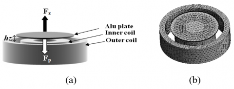
Figure 10 shows the electromagnetic levitation problem; TEAM workshop problem No. 28 [21]. The problem is made with a cylindrical aluminium plate of electrical conductivity σ=3.4E7S and m=0.107kg placed above two cylindrical coils. The inner coil has 960 turns while the outer coil has 576 turns. Both coils are electrically connected in series, but with inverse sense of winding. By this configuration, the plate is subject to an electromagnetic repulsion force Fz produced by eddy currents induced in this plate. This electromagnetic force can be expressed as following:
$\mathrm{Fz}=\mathbf{J}_{\text {ind}} \times \mathbf{B}$ (30)
Table 1. Comparison between the FVM solution and the analytical results
|
|
Electromagnetic Torque [Nm] |
Induced Voltage in The Phase Coil A [V] |
||
|
Angular Velocity [rad/s] |
Analytical Solution |
FVM Solution |
Analytical Solution |
FVM Solution |
|
0 |
3.83 |
3.70 |
0.63 |
0.58 |
|
200 |
6.50 |
6.47 |
0.84 |
0.76 |
|
400 |
-3.89 |
-3.88 |
1.48 |
1.42 |
|
600 |
-5.76 |
-5.96 |
0.76 |
0.68 |
|
800 |
-3.59 |
-3.96 |
0.62 |
0.57 |
|
1000 |
-2.70 |
-2.73 |
0.58 |
0.54 |
|
1200 |
-2.25 |
-2.73 |
0.56 |
0.53 |
Figure 7. Vectors of the magnetic flux density at 200rad/s
Figure 8. Eddy current density [A/m2] in the rotor at 200rad/s
Figure 9. Vectors of the electromagnetic force in the rotor
The aim here is to check the efficiency of the developed 3D FVM computer code associated to the prism mesh, that’s why we don’t take advantage of the axisymmetrical feature of the problem.
Figure 10. TEAM workshop problem No. 28 (a) Description, (b) Prism mesh
The solution of TEAM workshop problem No.28 requires the determination of the levitation height hz of the aluminium plate which refers to the distance between the lower edge of the plate and the upper edge of coils. In order to give the equilibrium position of the plate, i.e. equality of both electromagnetic force Fz and the weight force of the plate Fp, the solution of a correspondent inverse problem is carried out as shown in Figure 11.
Figure 11. Flowchart of the inverse problem
The algorithm of the inverse problem can be summarized as follows:
Step 0: Give an initial value of the levitation height hz(k), k=0.
Step 1: By using the direct electromagnetic formula i.e. Eq. 28, and for a given hz(k) we compute the electromagnetic force Fz(k) by Eq. 30.
Step 2: Check the convergence criterion of the inverse problem given by forces difference. If the convergence criterion is satisfied the iteration process is stopped, else the levitation height hz(k) is updated for the next inverse iteration k=k+1, and return to step (1).
Step 3: The levitation height of the aluminium plate hz(k) and the repulsive force Fz(k) are given by the last inverse iteration.
Table 2 shows a summary of the results. For each inverse iteration k, both the repulsive electromagnetic force Fz and the levitation height hz are computed. After eight inverse iterations, the difference ¶F becomes small enough and that is why the iteration process is stopped. As results, the aluminium plate is levitated with 11.84mm whereas the experimental value is 11.4mm [21].
Table 2. Summary of numerical results obtained by 3D FVM
|
Inverse iteration k |
Levitation hz[mm] |
Repulsive force Fz[N] |
|
1 2 3 4 5 6 7 8 |
15 7.5 11.25 13.13 12.19 11.72 11.95 11.84 |
0.59 2.12 1.17 0.84 0.99 1.08 1.03 1.06 |
|
Experimental levitation [mm] |
11.4 |
3.3 Electromagnetic micro-actuator
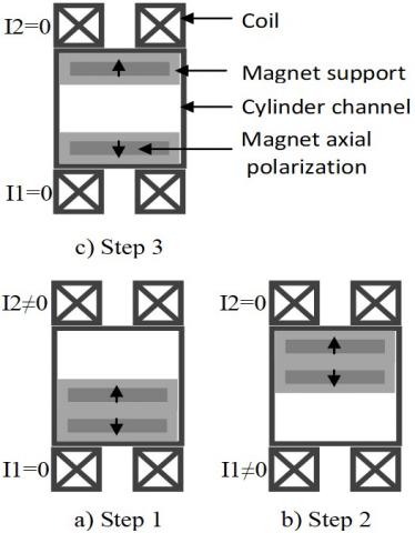
In this section, an experimental electromagnetic micro-actuator has been analyzed (Figure 12). The micro-actuator is made with two fixed identical coils and two permanent magnets. Each magnet is bonded to a non-magnetic material disc as a magnet support. In addition, the magnets are placed in opposite polarities. For more details on this micro-actuator as dimensions we refer to [22, 23].
Figure 12. The actuation steps of the micro-actuator
The actuating mode consists with moving vertically both permanent magnets inside a non-magnetic cylindrical channel. The magnetic force applied to magnets is generated by means the interaction of magnetic fields of both magnets and coils. The actuation is produced with a cyclical movement, where one cycle can be subdivided into three main actuation steps (Figure 12).
Let consider only the actuation of the upper magnet i.e. only the top coil will be supplied. Accordingly, only steps 1 and 3 are measured. In step 1, the top coil is supplied (I1=0, I2≠0) and thus a magnetic repulsive force is applied which drive the upper magnet to reach the lower one. In step 3, both coils are unsupplied (I1=I2=0) and hence a repulsive force between magnets drive the upper magnet to achieve the upper coil while the lower magnet still fixed to the lower coil.
The aim here is to simulate the actuation mode of the upper magnet by using the FVM method. The magnetic force applied to the upper magnet can be expressed as following:
$F_{z}=\int J_{a} \times B_{x}$ (31)
where, Ja is the equivalent fictive current of the upper magnet according to the Ampere’s approach:
$\mathbf{J}_{a}=\frac{\mathbf{B}_{r} \times \mathbf{n}}{\mu_{0}}$ (32)
In order to simulate the dynamic characteristic of the upper magnet i.e. magnet displacement versus time, the following mechanical equation is used:
$m \cdot \frac{\partial^{2} z}{\partial t^{2}}=F_{z}+m g$ (33)
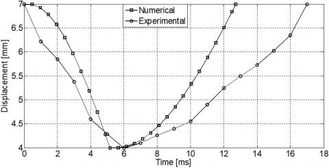
where, m and z are respectively the mass and the displacement of the upper magnet, and g is the gravity. Both numerical and experimental characteristics of the actuation are compared in Figure 13. Since frictions are not taken into account in the mechanical equation, the elapsed time in the numerical characteristic is less than in the experimental one with a difference of 4ms approximately. However, as in the two previous problems, the FVM method shows once more its effectiveness in the solution of problems related to electrodynamics.
Figure 13. Dynamic characteristic of the upper magnet
This paper presents the FVM as an alternative method for low frequency electromagnetic problems and in particular those require eddy current and electromagnetic force or torque computation. Both 2D and 3D computer codes are developed and tested. To examine the efficiency of both programs and showing the competitiveness of the FVM, both TEAM workshop problems No.28 and No.30 and an experimental electromagnetic micro-actuator are analyzed. One can see that numerical results obtained using the FVM are compared to the analytical or experimental results provided by these problems. Furthermore, the 3D FVM associated to the prism mesh can be a very promising for modelling problems without being constrained by their geometries.
|
Js |
Source current density |
|
Jind |
Eddy current density |
|
A |
Magnetic vector potential |
|
B |
Magnetic flux |
|
v |
Velocity |
|
Cem |
Electromagnetic torque |
|
Fz |
Electromagnetic force. |
|
hz |
Levitation height |
|
g |
Gravity |
|
m |
Mass |
|
Ci |
Geometrical and physical properties associated with the control volume |
|
Greek symbols |
|
|
$\mu$ |
Magnetic permeability |
|
$\sigma$ |
Electrical conductivity |
|
$\Omega_{p}$ |
Principal control volume of node P |
|
$v$ |
Magnetic reluctivity |
|
Subscripts |
|
|
FVM |
Finite volume method |
|
FEM |
Finite element method |
[1] Balborici, V., Dawson, F.P. (2016). Coupled circuit based representation of piezoelectric structures modeled using the finite volume method. Ultrasonics, 66: 103-110. https://doi.org/10.1016/j.ultras.2015.11.004
[2] Beckstein, P., Galindo, V., Vukčević, V. (2017). Efficient solution of 3D electromagnetic eddy-current problems within the finite volume framework of OpenFOAM. Journal of Computational Physics, 344: 623-646. http://dx.doi.org/10.1016/j.jcp.2017.05.005
[3] Berger, K., Quéval, L., Kameni, A., Alloui, L., Ramdane, B., Trillaud, F., Hell, L.M., Meunier, G., Masson, P., Lévêque, J. (2017). Benchmark on the 3D numerical modeling of a superconducting bulk. Hal.archives-ouvertes.fr/hal-01548728v4.
[4] Dong, G., Zou, J., Bayford, R.H., Ma, X., Gao, S., Yan, W., Ge, M. (2005). The comparison between FVM and FEM for EIT forward problem. IEEE Transactions on Magnetics, 41(5): 1468-1471. https//doi.org/10.1109/TMAG.2005.844558
[5] Cheriet, A., Zaoui, A., Feliachi, M., Mimoune, S.M. (2006). Computational performance comparison between FVM and FEM for 3-D magnetostatic problems. NUMELEC’06, 5eme Conférence Européenne sur les Méthodes Numériques en Electromagnétisme, Lille FRANCE, Proc, Art. 47.
[6] Deore, N., Chatterjee, A. (2010). A cell-vertex finite volume time domain method for electromagnetic scattering. Progress in Electromagnetics Research, 12: 1-15. https//doi.org/10.2528/PIERM10022003
[7] El Ghoul, I., Cheriet, A., Bensaid, S., Lakhdari, A. (2015). FVM model and virtual instrument based system for electromagnetic characterization of steel material. Journal of Applied Engineering Science & Technology, 2(2): 87-90.
[8] Gong, R., Ruan, J., Chen, J., Quan, Y., Wang, J., Jin, S. (2017). A 3-D coupled magneto-fluid-thermal analysis of a 220 kV three-phase three-limb transformer under DC bias. Energies, 10(4): 422. https://doi.org/10.3390/en10040422
[9] Laguna, A.A., Ozak, N., Lani, A., Deconinck, H., Poedts, S. (2018). Fully-implicit finite volume method for the ideal two-fluid plasma model. Computer Physics Communications, 231: 31-44. http://dx.doi.org/10.1016/j.cpc.2018.05.006
[10] Cioni, J.P., Remaki, M. (1997). Comparaison de deux méthodes de volumes finis en électromagnétisme. Research report No. 3166, INRIA Sophia Antipolis, France.
[11] Fumeaux, C., Baumann, D., Almpanis, G., Li, E.P., Vahldieck, R. (2008). Finite-volume time-domain method for electromagnetic modelling: Strengths, limitations and challenges. International Journal of Microwave and Optical Technology, 3(3): 318-328.
[12] Davies, J.B., Dean, A.J. (1996). Finite volume with non-uniform mesh for the solution of Maxwell's equations. IEEE Transactions on Magnetics, 32(3): 1417-1420. https//doi.org/10.1109/20.497513
[13] Zou, J., Yuan, J.S., Ma, X.S., Cui, X., Chen, S.M., He, J.L. (2004). Magnetic field analysis of iron-core reactor coils by the finite-volume method. IEEE Transactions on Magnetics, 40(2): 814-817. https//doi.org/10.1109/TMAG.2004.824773
[14] Cheriet, A., Feliachi, M., Mimoune, S.M. (2007). Nonconforming mesh generation for finite volume method applied to 3-D magnetic field analysis. The European Physical Journal Applied Physics, 37(2): 191-195. http://dx.doi.org/10.1051/epjap:2006152
[15] Hamimid, M., Mimoune, S.M., Feliachi, M. (2013). Incorporation of modified dynamic inverse Jiles-Atherton model in finite volume time domain for nonlinear electromagnetic field computation. Journal of Applied Physics, 113(1): 013915. http://dx.doi.org/10.1063/1.4773535
[16] Cheriet, A., Feliachi, M., Mimoune, S. (2009). 3-D movement simulation technique in FVM method application to eddy current non-destructive testing. COMPEL, 28(1): 77-84. http://dx.doi.org/10.1108/03321640910918887
[17] Li, Y., Torah, R., Beeby, S., Tudor, J. (2012). An all-inkjet printed flexible capacitor on a textile using a new poly (4-vinylphenol) dielectric ink for wearable applications. SENSORS, Taipei, pp. 1-4 https://doi.org/10.1155/2012/785271
[18] Mabrouk, A.E.H., Cheriet, A., Feliachi, M., Lakhdari, A.E. (2013). Transient axisymmetric FVM analysis of electodynamic levitation devices. The European Physical Journal Applied Physics, 61(1): 10602. http//doi.org/10.1051/epjap/2013120434
[19] Lepaul, S., Sykulski, J.K., Biddlecombe, C.S., Jay, A.P., Simkin, J. (1999). Coupling of motion and circuits with electromagnetic analysis. IEEE Transactions on Magnetics, 35(3): 1602-1605. https//doi.org/10.1109/20.767293