Hassanzadeh Merdad* | Metz Renaud | Mohamed Chaabane
© 2020 IIETA. This article is published by IIETA and is licensed under the CC BY 4.0 license (http://creativecommons.org/licenses/by/4.0/).
OPEN ACCESS
This paper presents a decentralized Takagi Sugeno (T-S) control scheme for a PV powered water pumping system, which is composed of a photovoltaic generator (PVG) supplying via a DC-DC boost converter, a DC-AC inverter, an Induction Motor coupled to a centrifugal pump. A T-S fuzzy controller is developed for MPPT (Maximum Power Point Tracking) to control the DC-DC boost converter, under variable solar irradiation and ambient temperature. An observer-based T-S fuzzy controller is dedicated to control the IM to guarantee the field-oriented control performances. From the optimal PV power provided in the MPP conditions, the optimal speed is calculated and delivered to control the IM, so that the proposed PV pumping system operates in optimal conditions and thus, maximizes the quantity of water pumped daily. Finally, simulation results are presented for both transient and steady state operation while taking into account all changes in climatic conditions, in order to validate the efficiency of the developed decentralized controller.
decentralized control, Induction Motor, MPPT, PV pumping system, T-S fuzzy control
Nowadays, recently and in a variety of countries, people suffer from the lack of potable water necessary to consume. Most of these countries are located in isolated areas where, conventional pumping systems is not a reliable solution, since that the electric power is not available. And, given the importance of this issue, renewable energy, specifically photovoltaic one, is integrated here to compensate the unavailability of electric power. Hence PV water pumping systems are considered as one of the most reliable remedy. More attention is dedicated to these operations’ design and implementation, in order to perform in a very reliable and economical way [1].
Different control strategies have been already developed for PV pumping systems; a dynamic performances analysis of a permanent magnet brushless DC (PMBLDC) motor is developed; proportional integral (PI) and a fuzzy logic (FL) speed controller are presented [2]. Betka and Moussi [3] has presented an optimal operation of a direct photovoltaic pumping system based on an induction motor (IM). Also sliding mode control design to track the maximum power point (MPPT) for a photovoltaic pumping system is proposed by Ellouze et al. [4], and Ameziane et al. [5].
There are a variety of motor pump unit configurations that are applied to PV pumping systems. Depending on the required application, the pumping system can be based on, submersible and surface or floating pumps types [6]. The commonly used pump is the centrifugal pump. This type of pump, the movement of the water through the pipe is assured by the impeller’s rotation, while equally depending on the total head of the water and the obtained mechanical power.
Likewise, the pump type, both AC and DC motors are used for the PV pumping systems. As it is frequently known about the DC motor, it indicates the disadvantage of brushes maintenance cost [7] which permits to permanent magnet brushless DC motors to be introduced in some applications [8]; but the PMBLDC motor is still not the best because of its high cost and its complicated hardware. Recent researches in AC motors made the (IM) an attractive and a worth option to take into consideration for the AC motors-based pumping setups [8].
Lately, the Takagi-Sugeno (T-S) approach is deemed to be a very effective method for modeling non-linear systems. It is based on the decomposition of the dynamic system behavior into different operation areas, that each one is presented by a local linear sub-model, in order to reduce the complexity of modeling task. These local sub-models are contributed through IF-THEN rules to the T-S global model, which is obtained by the interpolation of all sub-models [9-11].
In recent years, the design of decentralized controllers has been studied for large scale systems, due to the physical configuration and high dimensionality of this kind of system; which makes centralized control is neither economically feasible nor even necessary.
Since power systems are modelled as large-scale nonlinear systems, much effort has been focused on the application of decentralized control for these kind of systems [12, 13]. Particularly, a robust decentralized excitation control scheme is proposed for multimachine power system transient stability enhancement [14]. This work is divided into eliminating the nonlinearities of the multimachine power system at first and then developing a robust decentralized controller in order to guarantee the stability of the whole system. Bian et al. [15], Jian and Jiang [16] presented an adaptive decentralized control for large scale systems with unknown parameters and dynamic uncertainties with an application to power systems. By using the theory of robust adaptive dynamic programming (RADP), a decentralized optimal control design is given for large-scale systems with unmatched uncertainties.
In this paper we will develop a trajectory tracking decentralized control law for controlling both the boost converter and the induction motor using the multi-models fuzzy T-S technique. The aim of the proposed decentralized control is to decompose the global large-scale system (PV pumping system) into two sub-systems. Thus, the controller synthesis is equally divided into two local controllers in a way that for each sub-system is associated a local independent controller. First, T-S fuzzy controller is developed to insure the MPPT of the PV conversion first sub-system. In the other hand, the control of real large-scale systems, makes it unreasonable to assume that all states are measured, therefor an observer-based T-S fuzzy controller is designed which consists in reconstructing the inaccessible variables required for the IM. The control method, for both systems is based on a reference model to specify the desired trajectory, and it is based on the minimization of the effect of the disturbances on the tracking error according to the criterion H∞. For the stability phase, the control strategy adopted is based on the Lyapunov theory to guarantee a performant trajectory tracking. Hence, stability conditions are formulated as linear matrix inequalities (LMI).
The main contributions of this paper can be highlighted as follows: (1) Based on T-S fuzzy model, a H∞ decentralized control approach is designed to ensure that the whole system is asymptotically stable while rejecting external perturbations. (2) For the second observer-based T-S fuzzy controller, a one-step algorithm is proposed and formulated as an optimization problem in terms of matrix inequality, in order to give the observer and controller gains on a single step.
Figure 1. Photovoltaic pumping system
The above Figure 1 presents the structure of the proposed PV pumping system which is composed of the first subsystem: PV panel connected to a boost converter; a T-S fuzzy controller is developed to ensure the MPPT, and a second subsystem: an inverter connected to the unit motor-pump (centrifugal pump); equally a T-S fuzzy controller is dedicated for trajectory tracking under variable solar irradiation and ambient temperature.
2.1 PV conversion system
2.1.1 PV module
In the case of high-power applications and in order to reach the desired voltage and current levels, solar modules are electrically wired together to obtain a continuous electric source known as a photovoltaic generator (PVG). In this work, the PVG used is composed of 10 LC120P solar panels connected in series. Its parameters are presented in the Table 1.
Table 1. LC120-12P module
|
Parameters |
Abbreviations |
Values |
|
Maximum power Maximum current Maximum voltage Short circuit current Open circuit voltage |
Ppvopt Ipvopt Vpvopt Iph Voc |
120W 7A 17.1V 7.7A 21.8V |
Figure 2. Solar cell equivalent circuit
According to the above Figure 2, the photovoltaic current is given by the following expression:
$I_{p v}=I_{p h}-I_{0}\left(\exp \left(\frac{I_{p v}+R_{s} I_{p v}}{n V_{T}}\right)-1\right)-\left(\frac{V_{p v}+R_{s} I_{p v}}{R_{s h}}\right)$ (1)
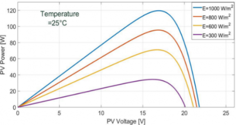
where, VT=KT/q; K is the Boltzmann constant, T is the cell temperature, q is the elementary charge, RS and Rsh are series and parallel resistances, respectively, I_ph is the generated photo current depending on the insolation and temperature changes and I_0 represents the diode’s saturation current. The following Figure 3 indicates the Power–Voltage (P-V) characteristic of the PV module. The curve shows the location of the MPP of the PV panel under various values of solar irradiation and constant cell temperature (25℃).
Figure 3. Characteristics of the PV module for various values of insolation
2.1.2 DC/DC boost converter modeling
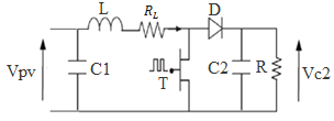
Figure 4 shows the basic circuit topology of the DC-DC boost converter. Its dynamic can be expressed with a linear differential equation that correspond to two phases: the store phase of electrical energy in the inductor (the switch is ON) and the transfer phase of energy (the switch is OFF). This leads to an average model as follows:
$\begin{aligned} \dot{x_{1}}(t)=&\left[A_{11} x_{1}(t)+E_{1} w_{1}(t)\right] u(t) \\ &+\left[A_{12} x(t)+E_{1} w_{1}(t)\right](1-u(t)) \end{aligned}$ (2)
As well,
$\dot{x_{1}}(t)=A_{12} x_{1}(t)+\left(A_{11}-A_{12}\right) x_{1}(t) u(t)$$+E_{1} w_{1}(t)$ (3)
$\dot{x_{1}}(t)=A_{12} x_{1}(t)+B_{1}\left(x_{1}(t)\right) u(t)+E_{1} w_{1}(t)$ (4)
where, $u(t) \in[0,1]$
$A_{11}=\left(\begin{array}{ccc}0 & -\frac{1}{c_{1}} & 0 \\ \frac{1}{L} & -\frac{R_{L}}{L} & 0 \\ 0 & 0 & -\frac{1}{R C_{2}}\end{array}\right)$; $A_{12}=\left(\begin{array}{ccc}0 & -\frac{1}{c_{1}} & 0 \\ \frac{1}{L} & -\frac{R_{L}}{L} & -\frac{1}{L} \\ 0 & \frac{1}{C_{2}} & -\frac{1}{R C_{2}}\end{array}\right)$;
$E_{1}=\left(\begin{array}{c}\frac{1}{C_{1}} \\ 0 \\ 0\end{array}\right)$ $x_{1}(t)=\left(\begin{array}{c}V_{p v}(t) \\ I_{L}(t) \\ V_{c 2}(t)\end{array}\right)$ $w_{1}(t)=I_{p v}(t)$
where, $B_{1}\left(x_{1}(t)\right)=\left(\begin{array}{c}0 \\ \frac{V_{c 2}(t)}{L} \\ -\frac{I_{L}(t)}{C_{2}}\end{array}\right)$ and u(t) defines the duty cycle.
Figure 4. DC/DC boost converter
2.1.3 MPPT searching algorithm
The MPPT algorithm adapted in our work, is based on the instant computation of the partial derivative of PV power with respect to the PV current. The MPP searching bloc gets the insolation and the temperature as inputs and provides the optimal values of PV voltage and current. At a maximum power point, the following condition is verified [11]:
$\frac{d}{d I_{p v}}\left(V_{p v} I_{p v}\right)=0$ (5)
Therefore,
$V_{p v}+I_{p v} \frac{d V_{p v}}{d I_{p v}}=0$ (6)
For maximum values of PV current and voltage, the value of PV power is maximum. By substituting Vpvopt and $\frac{d V_{p v}}{d I _{p v}}$ by their values in in the above equation, we obtain the following equation:
$\frac{2 R_{s}}{n V_{T}} I_{\text {pvopt}}-\left(I_{p h}-I_{\text {pvopt}}+I_{0}\right) Ln \left(\frac{I_{p h}-I_{\text {pvopt}}+I_{0}}{I_{0}}\right)=0$ (7)
The previous equation is solved for Ipvopt and indicates that this latter is proportionally dependent on the cell photocurrent Iph:
$I_{ {pvopt}}=0.9091 I_{p h}$ (8)
2.1.4 T-S fuzzy model for boost converter
The Takagi-Sugeno models are considered as universal approximators that ensure the perfect description of the dynamic behavior of nonlinear systems. The premise variables $z_{1 k}(t)=x_{1 k}(t) \in\left[z_{1 k, \min }, z_{1 k, \min }\right], k=1,2$ of the PV system are chosen as follow:
$\left\{\begin{array}{c}z_{11}(t)=V_{c 2}(t) \\ z_{12}(t)=I_{L}(t)\end{array}\right.$
Thus, the membership functions are defined by the following expressions:
$F_{1 k, \min }(z(t))=\frac{z_{1 k}(t)-z_{1 k, \min }}{z_{1 k, \max }-z_{1 k, \min }}$
$F_{1 k, \max }(z(t))=1-F_{1 k, \min }(z(t))$
The weighting functions of the derived T-S model are given by:
$\begin{aligned} h_{1}(z(t)) &=F_{11, \min }(z(t)) * F_{12, \min }(z(t)) \\ h_{2}(z(t)) &=F_{11, \min }(z(t)) * F_{12, \max }(z(t)) \\ h_{3}(z(t)) &=F_{11, \max }(z(t)) * F_{12, \min }(z(t)) \\ h_{4}(z(t)) &=F_{11, \max }(z(t)) * F_{12, \max }(z(t)) \end{aligned}$
Eventually, the overall output of the fuzzy rule-based system is given by:
$\dot{x_{1}}(t)=\sum_{i=1}^{4} h_{i}(z(t))\left(A_{12} x_{1}(t)+B_{1 i} u_{1}(t)+E_{1} w_{1}(t)\right)$ (9)
$B_{11}=\left(\begin{array}{c}0 \\ \frac{V_{c 2 \min }(t)}{L} \\ \frac{I_{L \min }(t)}{C_{2}}\end{array}\right)$; $B_{12}=\left(\begin{array}{c}0 \\ \frac{V_{C 2 \min }(t)}{L} \\ \frac{I_{L \max }(t)}{C_{2}}\end{array}\right)$
$B_{13}=\left(\begin{array}{c}0 \\ \frac{V_{C 2 \max }(t)}{L} \\ \frac{I_{{Lmin}}(t)}{C_{2}}\end{array}\right)$; $B_{14}=\left(\begin{array}{c}0 \\ \frac{V_{C 2 \max }(t)}{L} \\ \frac{I_{{Lmax}}(t)}{C_{2}}\end{array}\right)$
2.1.5 T-S fuzzy reference model
The goal to reach from this work is to elaborate a T-S fuzzy controller capable of ensuring the tracking of an optimal reference model which will produce the appropriate reference state to track. The equation of the MPP reference model in the state form can be written as follow [11]:
$\dot{x}_{1 r}(t)=A_{1 r} x_{1 r}(t)+r_{1}(t)$ (10)
where,
$A_{1 r}=\left(\begin{array}{ccc}0 & -\frac{1}{C_{1}} & 0 \\ \frac{1}{L} & -\frac{R_{L}}{L} & -\frac{1}{L}\left(1-u_{o p t}\right) \\ 0 & \frac{1}{C_{2}}\left(1-u_{o p t}\right) & -\frac{1}{R C_{2}}\end{array}\right)$
$u_{o p t}=\sqrt{\frac{V_{p v o p t}}{R I_{p v o p t}}}$
The reference model (10) is also nonlinear via the premise variable $z_{1 r}=\left(1-u_{o p t}\right)$. Thereby, the membership functions are presented by the following expressions:
$N_{1 \min }\left(z_{1 r}(t)\right)=\frac{z_{1 r}(t)-z_{1 r, \min }}{z_{1 r, \max }-z_{1 r, \min }}$
The matrices of the reference model are defined as:
$A_{11 r}=\left(\begin{array}{ccc}0 & -\frac{1}{C_{1}} & 0 \\ \frac{1}{L} & -\frac{R_{L}}{L} & -\frac{1}{L} z_{r, \min } \\ 0 & \frac{1}{C_{2}} z_{r, \min } & -\frac{1}{R C_{2}}\end{array}\right)$
$A_{12 r}=\left(\begin{array}{ccc}0 & -\frac{1}{C_{1}} & 0 \\ \frac{1}{L} & -\frac{R_{L}}{L} & -\frac{1}{L} z_{r, \max } \\ 0 & \frac{1}{C_{2}} z_{r, \max } & -\frac{1}{R C_{2}}\end{array}\right)$
As so, the global T-S fuzzy reference model is:
$\dot{x}_{1 r}(t)=\sum_{k=1}^{2} h_{k}\left(z_{1 r}(t)\right)\left(A_{1 k r} x_{1 r}(t)+r_{1}(t)\right)$ (11)
2.1.6 T-S fuzzy controller
This section is dedicated to develop the control laws which are also based on the T-S fuzzy modeling. Here, we adopted the same principle of the ordinary PDC controller but in addition, in the control law, we take into account the term of the tracking error: $e_{1 r}(t)=\left(x_{1}(t)-x_{1 r}(t)\right)$. As mentioned before, the objective is that, in spite of the change in the insolation values, the system needs to function in the optimum operating conditions which are characterized by a tracking error converging to zero. Thus, the trajectory tracking issue is formulated as a fuzzy state feedback control given by:
$u_{1}(t)=\sum_{j=1}^{4} h_{j}(z(t)) K_{1 j}\left(e_{1 r}(t)\right)$ (12)
where, K1j are the controller gains to calculate later.
By replacing each of the reference state (11), the system real state (9) and the control law (12) by their expressions, we obtain the error dynamics as:
$e_{1 r}^{\cdot}(t)$$=\sum_{i=1}^{4} \sum_{j=1}^{4} \sum_{k=1}^{2} h_{i}(z(t)) h_{j}(z(t)) h_{k}\left(z_{r}(t)\right)$
$\times\left[\begin{array}{c}\left(A_{12}+B_{1 i} K_{1 j}\right) e_{1 r}(t)+ \left(A_{12}-A_{1 k r}\right) x_{r 1}(t)+E_{1} w_{1}(t)-r_{1}(t)\end{array}\right]$ (13)
Thus, by injection the above expression in the overall T-S fuzzy model (9), the following augmented state-space form is obtained:
$\dot{\bar{{x}_{1}}}(t)=\sum_{i=1}^{4} \sum_{i=1}^{4} \sum_{k=1}^{2} h_{i}(z(t)) h_{j}(z(t)) h_{k}\left(z_{1 r}(t)\right)\times\left[\bar{A}_{i j k} \overline{x_{1}}(t)+\overline{E_{1}} \overline{w_{1}}(t)\right]$ (14)
where,
$\begin{aligned} \overline{x_{1}}(t)=&\left[\begin{array}{l}e_{r 1}(t) \\ x_{1 r}(t)\end{array}\right] \quad \overline{w_{1}}(t)=\left[\begin{array}{c}w_{1}(t) \\ r_{1}(t)\end{array}\right] \quad \overline{E_{1}}=\left[\begin{array}{cc}E_{1} & -I \\ 0 & I\end{array}\right] \\ \bar{A}_{i j k} &=\left[\begin{array}{cc}A_{12}+B_{1 i} K_{1 j} & A_{12}-A_{1kr} \\ 0 & A_{1 k r}\end{array}\right] \end{aligned}$
r1(t) is the external input depending on the insolation and the temperature and W1(t) designates the external disturbance.
The H∞ performance is added to the closed-loop control system in the purpose of attenuating the external disturbance’s effect; it is expressed as follow:
$\int_{0}^{t f} \overline{x_{1}}^{T}(t) \overline{Q_{1}} \overline{x_{1}}(t) d t \leq \rho_{1}^{2} \int_{0}^{t f} \overline{w_{1}}^{T}(t) \overline{w_{1}}(t) d t$ (15)
where, $\overline{Q_{1}}=\left[\begin{array}{ll}Q_{1} & 0 \\ 0 & 0\end{array}\right]$ is a positive definite weighting matrix and ρ1 is a prescribed attenuation level against the external disturbance effect.
2.2 Induction Motor modeling and control
To elaborate the electromagnetic dynamics of the IM, we are looking to determine the biphasic model of the machine in the synchronously d-q reference frame, in order to facilitate its study. In this context, these hypotheses are adopted:
The magnetic circuit is linear.
The permeability of the magnetic circuit is assumed to be infinite and iron losses are not taken into account.
The mechanical losses are neglected.
The air gap thickness is constant while the notch effect is neglected.
2.2.1 Mathematical model in d-q coordinates
The dynamic model of the IM in the synchronous biphase d-q reference frame can be formulated as follow [17]:
$\dot{x_{2}}(t)=f_{2}\left(x_{2}(t)\right)+g_{2}\left(x_{2}(t)\right) u_{2}(t)+w_{2}(t)$ (16)
$g_{2}\left(x_{2}(t)\right)=\left[\begin{array}{ccccc}\frac{1}{\sigma L_{s}} & 0 & 0 & 0 & 0 \\ 0 & \frac{1}{\sigma L_{s}} & 0 & 0 & 0\end{array}\right]^{T}$; $u_{2}(t)=\left[\begin{array}{ll}u_{s d} & u_{s q}\end{array}\right]^{T}$
$x_{2}(t)=\left[\begin{array}{lllll}i_{s d} & i_{s q} & \psi_{r d} & \psi_{r q} & w_{m}\end{array}\right]^{T}$
$w_{2}(t)=\left[\begin{array}{lllll}0 & 0 & 0 & 0 & -\frac{C_{r}}{J}\end{array}\right]^{T}$
$f_{2}\left(x_{2}(t)\right)=\left[\begin{array}{c}-\alpha i_{s d}+w_{s} i_{s q}+\frac{K_{s}}{T_{r}} \psi_{r d}+K_{s} n_{p} w_{m} \psi_{r q} \\ -w_{s} i_{s d}-\alpha i_{s q}-K_{s} n_{p} w_{m} \psi_{r d}+\frac{K_{s}}{T_{r}} \psi_{r q} \\ \frac{M}{T_{r}} i_{s d}-\frac{1}{T_{r}} \psi_{r d}+\left(w_{s}-n_{p} w_{m}\right) \psi_{r q} \\ \frac{M}{T_{r}} i_{s q}-\left(w_{s}-n_{p} w_{m}\right) \psi_{r d}-\frac{1}{T_{r}} \psi_{r q} \\ \frac{n_{p} M}{J L_{r}}\left(\psi_{r d} i_{s q}-\psi_{r q} i_{s d}\right)-\frac{f}{J} w_{m}\end{array}\right]$
$\alpha=\left(\frac{1}{\sigma T_{s}}+\frac{1-\sigma}{\sigma T_{r}}\right) ; K_{S}=\frac{M}{\sigma L_{s} L_{r}} ; T_{r}=\frac{L_{r}}{R_{r}} ; T_{s}=\frac{L_{s}}{R_{s}}; \sigma=1-\frac{M^{2}}{L_{s} L_{r}}$
where, ws is the electrical speed of stator, wm is the rotor speed, (usd;usq) are the direct and quadratic voltages of the stator, (isd;isq) are the stator currents and (ψrd;ψrq) are the flux of the rotor, Cr is the load torque, J is the moment of inertia, (Rs;Rr) are the rotor and stator resistances, (Ls;Lr) are the rotor and stator inductances, M is the mutual-inductance, f is the friction coefficient and np is the number of pole pairs.
2.2.2 Open loop control strategy
In this section we adopted the principle of rotor flow orientation for the open loop control, it ensures a natural decoupling between the stator current isd and the rotor flux ψrd and between the stator current isq and the electromagnetic torque Cem. By replacing the state variables $x_{2}(t)=\left[\begin{array}{lllll}i_{s d c} & i_{s q c} & \psi_{r d c} & \psi_{r q} & w_{m c}\end{array}\right]^{T}$ of the machine $\begin{array}{llll}\text { by } & \text { its } & \text { reference } & \text { corresponding } & \text { ones } & x_{2 r}(t)=\end{array}$ $\left[\begin{array}{lllll}i_{s d c} & i_{s q c} & \psi_{r d c} & 0 & w_{m c}\end{array}\right]^{T}$ in $(16),$ we obtain the following model:
$\left\{\begin{array}{c}\frac{d}{d t} i_{s d c}=-\alpha i_{s d c}+w_{s} i_{s q c}+\frac{K_{s}}{T_{r}} \psi_{r d c}+\frac{1}{\sigma L_{s}} u_{s d c} \\ \frac{d}{d t} i_{s q c}=-w_{s} i_{s d c}-\alpha i_{s q c}-K_{s} n_{p} w_{m c} \psi_{r d c}+\frac{1}{\sigma L_{s}} u_{s q c} \\ \frac{d}{d t} \psi_{r d c}=\frac{M}{T_{r}} i_{s d c}-\frac{1}{T_{r}} \psi_{r d c} \\ 0=\frac{M}{T_{r}} i_{s q c}-\left(w_{s}-n_{p} w_{m c}\right) \psi_{r d c} \\ \frac{d}{d t} w_{m c}=\frac{n_{p} M}{J L_{r}}\left(\psi_{r d c} i_{s q c}\right)-\frac{f}{J} w_{m c}-\frac{c_{r}}{J}\end{array}\right.$ (17)
From the above system, we extract the reference stator current, the reference electrical speed and the open-loop control law:
$\left\{\begin{array}{c}i_{s d c}=\frac{\psi_{r d c}}{M}+\frac{T_{r}}{M} \frac{d}{d t} \psi_{r d c} \\ i_{s q c}=\frac{J L_{r}}{n_{p} M \psi_{r d c}}\left(\frac{C_{r}}{J}+\frac{f}{J} w_{m c}+\frac{d}{d t} w_{m c}\right)\end{array}\right.$ (18)
$w_{s c}=n_{p} w_{m c}+\frac{M}{T_{r} \psi_{r d c}} i_{s q c}$ (19)
$\left\{\begin{array}{c}u_{s d c}=\sigma L_{s}\left(\frac{d}{d t} i_{s d c}+\alpha i_{s d c}-w_{s c} i_{s q c}-\frac{K_{s}}{T_{r}} \psi_{r d c}\right) \\ u_{s q c}=\sigma L_{s}\left(\frac{d}{d t} i_{s q c}+\alpha i_{s q c}+w_{s c} i_{s d c}+K_{s} n_{p} w_{m c} \psi_{r d c}\right)\end{array}\right.$ (20)
2.2.3 T-S fuzzy model of the Induction Motor
When the field-oriented strategy is implemented, the dynamics of the IM is similar to the separately excited DC motor and the electrical stator speed is expressed in the synchronously rotating frame as:
$w_{s}=n_{p} w_{m}+\frac{M}{T_{r} \psi_{r d c}} i_{s q}$ (21)
Thus, the nonlinear model of the IM may be given as the state space form:
$\left\{\begin{array}{c}\dot{x_{2}}(t)=A_{2} x_{2}(t)+B_{2} u_{2}(t)+w_{2}(t) \\ y_{2}(t)=C_{2} x_{2}(t)\end{array}\right.$ (22)
$A_{2}\left(x_{2}(t)\right)=\left[\begin{array}{ccccc}-\alpha & w_{s} & \frac{K_{s}}{T_{r}} & K_{s} n_{p} w_{m} & 0 \\ -w_{s} & -\alpha & -K_{s} n_{p} w_{m} & \frac{K_{s}}{T_{r}} & 0 \\ \frac{M}{T_{r}} & 0 & -\frac{1}{T_{r}} & \frac{M}{T_{r} \psi_{r d c}} i_{s q} & 0 \\ 0 & \frac{M}{T_{r}} & -\frac{M}{T_{r} \psi_{r d c}} i_{s q} & -\frac{1}{T_{r}} & 0 \\ 0 & 0 & \frac{n_{p} M}{J_{r}} i_{s q} & -\frac{n_{p} M}{J L_{r}} i_{s d} & -\frac{f}{J}\end{array}\right]$
$B_{2}=\left[\begin{array}{ccccc}\frac{1}{\sigma L_{s}} & 0 & 0 & 0 & 0 \\ 0 & \frac{1}{\sigma L_{s}} & 0 & 0 & 0\end{array}\right]^{T}$
$C_{2}=\left[\begin{array}{lllll}1 & 0 & 0 & 0 & 0 \\ 0 & 1 & 0 & 0 & 0 \\ 0 & 0 & 0 & 0 & 1\end{array}\right] ; w_{2}(t)=\left[\begin{array}{lllll}0 & 0 & 0 & 0 & -\frac{C_{r}}{J}\end{array}\right]^{T}$
$A_{2}\left(x_{2}(t)\right)$ includes nonlinear terms $z_{2 k}(t)=x_{2 k}(t) \in$ $\left[z_{2 k m i n}, z_{2 k m a x}\right]$ with $k=1,2,3,$ as follow:
$\left\{\begin{array}{l}z_{21}(t)=i_{s d}(t) \\ z_{22}(t)=i_{s q}(t) \\ z_{23}(t)=w_{m}(t)\end{array}\right.$ (23)
Thus, the membership functions corresponding to the premise variables (23) are:
$\left\{\begin{array}{c}F_{2 k, \min }\left(z_{k}(t)\right)=\frac{z_{2 k}(t)-z_{2 k, \min }}{z_{2 k, \max }-z_{2 k, \min }} \\ F_{2 k, \max }\left(z_{k}(t)\right)=1-F_{2 k, \min }\left(z_{2 k}(t)\right)\end{array}\right.$ (24)
The global fuzzy model is inferred as follows:
$\dot{x_{2}}(t)=\sum_{i=1}^{8} \theta_{i}(z(t))\left(A_{2 i} x_{2}(t)+B_{2} u_{2}(t)+w_{2}(t)\right)$ (25)
where,
$\left\{\begin{aligned} \theta_{i}(z(t))=& \frac{\lambda_{i}(z(t))}{\sum_{i=1}^{8} \lambda_{i}(z(t))} ; \lambda_{i}(z(t))=\prod_{k=1}^{3} F_{2 i, k}\left(z_{2 k}(t)\right) \\ & \theta_{i}(z(t))>0 ; \sum_{i=1}^{8} \lambda_{i}(z(t))=1 \end{aligned}\right.$
$\theta_{i}(z(t))$ is the normalized weight of the i-rule, and $F_{2 i, k}\left(z_{2 k}(t)\right)$ is the grade of membership of $z_{2 k}(t)$ in $F_{2 i, k}$.
2.2.4 T-S fuzzy reference model for Induction Motor
Basing on the same previous principle, the T-S fuzzy reference model will generate the desired trajectory to be tracked by the state variables of the machine. A positive parameter K_i is inserted in the model, in order to improve the transient performance of the closed-loop system. The new control input vector is defined as follow [18]:
$\left\{\begin{array}{l}u_{s d c}^{\prime}=u_{s d c}+K_{i} \sigma L_{s}\left(i_{s d c}-i_{s d r}\right) \\ u_{s q c}^{\prime}=u_{s q c}+K_{i} \sigma L_{s}\left(i_{s q c}-i_{s q r}\right)\end{array}\right.$ (26)
$\left\{\begin{array}{c}u_{s d c}=\sigma L_{s}\left(\frac{d i_{s d c}}{d t}+\alpha i_{s d c}-w_{s c} i_{s q c}-\frac{K_{s}}{T_{r}} \psi_{d r c}\right) \\ u_{s q c}=\sigma L_{s}\left(\frac{d i_{s q c}}{d t}+\alpha i_{s q c}+w_{s c} i_{s d c}+K_{s} n_{p} w_{m c} \psi_{d r c}\right)\end{array}\right.$ (27)
The system (28) can be rewritten as:
$\left\{\begin{array}{c}u_{s d c}^{\prime}=\sigma L_{s}\left[\frac{d i_{s d c}}{d t}+\left(\alpha+K_{i}\right) i_{s d c}-w_{s c} i_{s q c}-\frac{K_{s}}{T_{r}} \psi_{d r c}-K_{i} \sigma L_{s} i_{s d r}\right] \\ u_{s q c}^{\prime}=\sigma L_{s}\left[\frac{d i_{s q c}}{d t}+\left(\alpha+K_{i}\right) i_{s q c}+w_{s c} i_{s d c}+K_{s} n_{p} w_{m c} \psi_{d r c} -K_{i} \sigma L_{s} i_{s q r}\right]\end{array}\right.$ (28)
Also,
$\left\{\begin{array}{l}u_{s d c}^{\prime}=u_{s d r}-K_{i} \sigma L_{s} i_{s d r} \\ u_{s q c}^{\prime}=u_{s q r}-K_{i} \sigma L_{s} i_{s q r}\end{array}\right.$ (29)
The state equation of the reference model of the IM is:
$\dot{x}_{2 r}(t)=A_{2 r} x_{2 r}(t)+r_{2}(t)$ (30)
where,
$\left(x_{2}(t)\right)=\left[\begin{array}{ccccc}-\xi_{1} & w_{s r} & \frac{K_{s}}{T_{r}} & K_{s} n_{p} w_{m r} & 0 \\ -w_{s r} & -\xi_{1} & -K_{s} n_{p} w_{m r} & \frac{K_{s}}{T_{r}} & 0 \\ \frac{M}{T_{r}} & 0 & -\frac{1}{T_{r}} & \frac{M}{T_{r} \psi_{r d c}} i_{s q r} & 0 \\ 0 & \frac{M}{T_{r}} & -\frac{M}{T_{r} \psi_{r d c}} i_{s q r} & -\frac{1}{T_{r}} & 0 \\ 0 & 0 & \frac{n_{p} M}{J_{r}} i_{s q r} & -\frac{n_{p} M}{J L_{r}} i_{s d r} & -\frac{f}{J}\end{array}\right]$
$\xi_{1}=\alpha+K_{i} ; w_{s r}=n_{p} w_{m r}+\frac{M}{T_{r} \psi_{r d c}} i_{s q r}$;
and $r_{2}(t)=\left[\begin{array}{cc}B_{2} & I\end{array}\right]\left[\begin{array}{c}u_{2 r} \\ w_{2}(t)\end{array}\right] ;$ where $u_{2 r}(t)=\left[\begin{array}{l}u_{s d r} \\ u_{s q r}\end{array}\right]$
The measurable premise variables are defined as:
$\left\{\begin{array}{l}z_{21 r}(t)=i_{s d r}(t) \\ z_{22 r}(t)=i_{s q r}(t) \\ z_{23 r}(t)=w_{m r}(t)\end{array}\right.$
The overall fuzzy reference model is given by:
$\dot{x}_{2 r}(t)=\sum_{j=1}^{8} \theta_{r j}\left(z_{2 r}(t)\right) A_{2 j r} x_{2 r}(t)+r_{2}(t)$ (31)
The H∞ performance related to the tracking error $e_{2 r}(t)=x_{2 r}(t)-x_{2}(t)$ is presented by the following inequality:
$\int_{0}^{t_{f}}\left[\left(x_{2 r}(t)-x_{2}(t)\right)^{T} Q_{2}\left(x_{2 r}(t)-x_{2}(t)\right)\right] d t \leq$
$\rho_{2}^{2} \int_{0}^{t_{f}}\left[\left(r_{2}(t)^{T} r_{2}(t)+w_{2}(t)^{T} w_{2}(t)\right] d t\right.$ (32)
r2(t) is the reference input, w2(t) is the external disturbance, Q2 is a positive definite weighting matrix and ρ2 is the attenuation level.
2.2.5 T-S fuzzy observer for Induction Motor
A Luenberger type multi-observer is constructed in this part to estimate the immeasurable state of the induction motor. Since the availability of all the variables is required, the T-S observer will to estimate the inaccessible rotor flux. As so, the T-S fuzzy observer is developed as so:
$\left\{\begin{array}{c}\dot{\hat{x}_{2}}(t)=\sum_{i=1}^{8} \theta_{i}(z(t))\left(A_{2 i} \hat{x}_{2}(t)+B_{2} u_{2}(t)\right. \\ \left.+L_{i}\left(y_{2}(t)-\hat{y}_{2}(t)\right)\right) \\ \hat{y}_{2}=C_{2} \hat{x}_{2}(t)\end{array}\right.$. (33)
$\hat{x}_{2}(t)$ and $\hat{y}_{2}(t)$ designate respectively the estimated state and output vectors, while Li are the observer gains.
We define the estimated error as $e_{2}(t)=x_{2}(t)-\hat{x}_{2}(t)$ for which the fuzzy model is given by:
$\dot{e}_{2}(t)=\sum_{i=1}^{8} \theta_{i}(z(t))\left[\left(A_{2 i}-L_{i} C_{2}\right) e_{2}(t)\right]+w_{2}(t)$ (34)
2.2.6 Tracking controller design
For the design of the observer-based controller, we adopted the same principle of the ordinary PDC controller but in addition, in the feedback control law, we take into account the reference state xr(t) as following:
$u_{2}(t)=\sum_{i=1}^{8} \theta_{i}(z(t)) K_{2 i}\left(\hat{x}_{2}(t)-x_{2 r}(t)\right)$ (35)
where, K2i are the fuzzy control gain and $e_{2 r}(t)=\hat{x}_{2}(t)-x_{2 r}(t)$ is the tracking error for which the fuzzy model is as:
$\dot{e}_{2 r}(t)=\sum_{i=1}^{8} \sum_{j=1}^{8} \theta_{i}(z(t))\left(\theta_{j}\left(z_{2 r}(t)\right)\left[\left(A_{2 i}+\right.\right.\right.$
$\left.B_{2} K_{2 j}\right) e_{2 r}(t)-B_{2} K_{2 j} e_{2}(t)+\left(A_{2 i}-\right.$$\left.\left.A_{2 j r}\right) x_{2 r}(t)\right]+w_{2}(t)-r_{2}(t)$. (36)
We obtain the following closed-loop system written in an augmented state-space form as:
$\dot{\bar{x}}_{2}(t)=\sum_{i=1}^{8} \sum_{j=1}^{8} \theta_{i}(z(t))\left(\theta_{j}\left(z_{2 r}(t)\right)\right.$ $\left.\times \overline{[G}_{i j} \bar{x}_{2}(t) \bar{E}_{2} \bar{w}_{2}(t)\right]$ (37)
$\bar{x}_{2}(t)=\left[\begin{array}{c}e_{2 r}(t) \\ e_{2}(t) \\ x_{2 r}(t)\end{array}\right] \quad \bar{w}_{2}(t)=\left[\begin{array}{c}w_{2}(t) \\ r_{2}(t)\end{array}\right] \quad \bar{E}_{2}=\left[\begin{array}{cc}I & -I \\ I & 0 \\ 0 & I\end{array}\right]$
$\bar{G}_{i j}=\left[\begin{array}{ccc}A_{2 i}+B_{2} K_{2 j} & -B_{2} K_{2 j} & A_{2 i}-A_{2 j r} \\ 0 & A_{2 i}-L_{i} C_{2} & 0 \\ 0 & 0 & A_{2 j r}\end{array}\right]$
Therefore, the H∞ tracking performance is reformulated as:
$\int_{0}^{t f} \overline{x_{2}}^{T}(t) \overline{Q_{2}} \overline{x_{2}}(t) d t \leq \rho_{2}^{2} \int_{0}^{t f} \overline{w_{2}}^{T}(t) \overline{w_{2}}(t) d t$ (38)
where, $\overline{Q_{2}}=\left[\begin{array}{lll}Q_{2} & 0 & 0 \\ 0 & 0 & 0 \\ 0 & 0 & 0\end{array}\right]$
The next part is dedicated to study the stability of the closed loop system while maintaining a good trajectory tracking performance.
2.2.7 Reference speed
In order to search the optimum operating speed corresponding to the maximum power delivered by the PVG for various values of temperature and insolation, a reference speed bloc is added to compute instantly the reference speed $w_{m_{o p t}}$ that should be tracked and which assures the optimal operating of the IM, and thus a significant part of the available solar power is transferred to the unit motor-pump.
First, we start by defining the electrical power equation absorbed by the IM:
$P_{a b s}=\frac{3}{2} *\left(u_{s d} * i_{s d}+u_{s q} * i_{s q}\right)$ (39)
Then, and by replacing usd, usq, usd, isd, and isq by their equations respectively (28) and (18), the DC electrical power will be expressed as a function of the motor speed in the following form as follow:
$P_{a b s}=C_{1}+C_{2} * w_{m o p t}^{2}+C_{3} * w_{m o p t}^{3}+C_{4} * w_{m o p t}^{4}$ (40)
$C_{1}=\sigma L_{S}\left(\frac{\psi_{r d}}{M}\right)^{2}\left(\alpha-K_{s} \frac{M}{T_{r}}\right)$
$C_{2}=\sigma L_{S}\left(\alpha K_{q}^{2} f^{2}+K_{s} K_{q} n_{p} f \psi_{r d}\right)$
$C_{3}=\sigma L_{S} A_{p}\left(2 \alpha K_{q}^{2} f+K_{s} K_{q} n_{p} \psi_{r d}\right)$
$C_{4}=\sigma L_{s} \alpha K_{q}^{2} A_{p}^{2} ; K_{q}=\frac{2 L_{r}}{3 n_{p} M \psi_{r d}}$
By assuming that the loses in DC converter is only in the inductance resistor RL, and in the case of reaching the maximum power point conditions of the PVG, the optimal motor speed wmopt can be obtained on-line by the Eq. (42) while adopting the following relation:
$P_{a b s}=P_{p v}-R_{L} * I_{p v}^{2}$ (41)
$w_{m_{o p t}}=\frac{P_{p v}-R_{L} * I_{p v}^{2}-C_{1}}{C_{2} * w_{m o p t}+C_{3} * w_{m o p t}^{2}+C_{4} * w_{m o p t}^{3}}$ (42)
2.3 Centrifugal pump
In this work, we used a centrifugal pump for which the characteristic H(Q) may be represented by:
$H=a Q^{2}+b Q w_{m}+c w_{m}^{2}$ (43)
H is the total head, Q designates the flow rate, wm is the speed and a, b and c are three constants that depends on the pump’s dimensions. The above equation relates the main parameters of the centrifugal pump, the flow rate, the head and the speed. The pump performance is predicted by specifying a load curve [20]:
$H=H_{g}+\Delta H$ (44)
Hg is the static height (the distance between the free level of water and the highest point of the canalization), and ∆H is the pressure losses in the canalization equal to:
$\Delta H=\frac{8\left(\frac{\partial l}{d}+\xi\right) Q^{2}}{\pi^{2} d^{4} g}$ (45)
where, ∂ is a resistance coefficient in the canalization, l is the length of the pipeline, d is the diameter of the pipeline, ξ is a local resistance coefficient and g is the gravity acceleration. Hence, the objective of this study is to determine a decentralised fuzzy controller with the H∞ tracking performance able to force the PV pumping system to operate very close to its maximum power trajectory for all climatic conditions’ variations. The main result is stated in the following two theorems.
Theorem 1: Considering the photovoltaic system (9). The closed-loop system (14) is asymptotically stable and the H∞ performance (15) with the attenuation level ρ is bounded, if there exist the following matrices $\mathrm{X}_{11}=\mathrm{P}_{11}^{-1}>0, \mathrm{P}_{12}>0, \mathrm{Y}_{1 \mathrm{i}}$ and a positive scalar ρ1 solution for the following optimization problem:
$\min _{\left(P_{11}, P_{12}\right)}\left(\rho_{1}\right)$
Subject to:
$\left[\begin{array}{cccccccc}\psi_{11} & \left(A_{12}-A_{1 k r}\right) & E_{1} & -I & 0 & 0 & 0 & X_{11} \\ * & -2 \mu_{1} X_{11} & 0 & 0 & -\mu_{1} I & 0 & 0 & 0 \\ * & * & -2 \mu_{1} & 0 & 0 & -\mu_{1} I & 0 & 0 \\ * & * & * & -2 \mu_{1} & 0 & 0 & -\mu_{1} I & 0 \\ * & * & * & * & \psi_{22} & 0 & P_{12} & 0 \\ * & * & * & * & * & -\rho_{1}^{2} I & 0 & 0 \\ * & * & * & * & * & * & -\rho_{1}^{2} I & 0 \\ * & * & * & * & * & * & * & -Q_{1}^{-1}\end{array}\right]<0$ (46)
where,
$Y_{i}=K_{1 i} X_{11} ; \psi_{22}=A_{1 k r}^{T} P_{12}+P_{12} A_{1 k r}$
$\psi_{11}=A_{12} X_{11}+X_{11} A_{12}^{T}+B_{1 i} Y_{1 j}+Y_{1 j}^{T} B_{1 i}^{T}$
μ1 is a scalar.
Theorem 2: For a positive scalar µ, the closed-loop system (37) is asymptotically stable and the H∞ performance (38) with the attenuation level ρ is bounded if there exist definite matrices $\mathrm{X}_{21}=\mathrm{P}_{21}^{-1}>0, \mathrm{P}_{22}>0, \mathrm{P}_{23}>0, \mathrm{Y}_{2 \mathrm{j}}, \mathrm{J}_{\mathrm{i}}$ and a positive scalar ρ2 solution for the following optimisation problem:
$\min _{\left(P_{21}, P_{22}\right)}\left(\rho_{2}\right)$
Subject to:
$\left[\begin{array}{ccccccccc}\varphi_{11} & -B_{2} K_{2 j} & A_{2 i}-A_{2 j r} & I & -I & 0 & 0 & 0 & 0 & X_{21} \\ * & -2 \mu_{2} X_{21} & 0 & 0 & 0 & \mu_{2} I & 0 & 0 & 0 & 0 \\ * & * & -2 \mu_{2} I & 0 & 0 & 0 & \mu_{2} I & 0 & 0 & 0 \\ * & * & * & -2 \mu_{2} I & 0 & 0 & 0 & \mu_{2} I & 0 & 0 \\ * & * & * & * & -2 \mu_{2} I & 0 & 0 & 0 & \mu_{2} I & 0 \\ * & * & * & * & * & \varphi_{22} & 0 & P_{22} & 0 & 0 \\ * & * & * & * & * & * & \varphi_{33} & 0 & P_{23} & 0 \\ * & * & * & * & * & * & * & -\rho_{2}^{2} I & 0 & 0 \\ * & * & * & * & * & * & * & * & -\rho_{2}^{2} I & 0 \\ * & * & * & * & * & * & * & * & * & -Q_{2}^{-1}\end{array}\right]<0 $ (47)
where,
$Y_{2 j}=K_{2 j} X_{21}^{-1} ; L_{i}=P_{22}^{-1} J_{i}$
$\varphi_{11}=A_{2 i} X_{21}+X_{21} A_{2 i}^{T}+B_{2} Y_{2 j}+Y_{2 j}^{T} B_{2}^{T}$
$\varphi_{22}=A_{2 i}^{T} P_{22}+P_{22} A_{2 i}-J_{i} C_{2}-C_{2}^{T} J_{2 i}^{T}$
$\varphi_{33}=P_{23} A_{2 j r}+A_{2 j r}^{T} P_{23}$
and μ2 is a scalar.
2.4 Global stability of PV pumping system
The stability of the global system is studied using the quadratic function of Lyapunov $V(\bar{x}(t))$ such that $\bar{P}_{i}$ is a positive definite symmetric matrix (i = 1,2) [19]:
$V(\bar{x}(t))=\bar{x}_{1}^{T}(t) \bar{P}_{1} \bar{x}_{1}(t)+\bar{x}_{2}^{T}(t) \bar{P}_{2} \bar{x}_{2}(t)$ (48)
The derivative of Lyapunov's function is written as:
$\dot{V}(\bar{x}(t))=\dot{\bar{x}_{1}^{T}}(t) \bar{P}_{1} \bar{x}_{1}(t)+\bar{x}_{1}^{T}(t) \bar{P}_{1} \dot {\bar{{x}_{1}}}(t)+\dot{\bar{x}_{2}^{T}}(t) \bar{P}_{2} \bar{x}_{2}(t)+\bar{x}_{2}^{T}(t) \bar{P}_{2} \dot{\bar{x}}_{2}(t)$ (49)
According to the H∞ tracking performances (15) and (38), and in order to realize the stability of the global pumping system, the following inequality must be verified:
$\dot{V}(\bar{x}(t))+\bar{x}_{1}^{T}(t) \bar{Q}_{1} \bar{x}_{1}(t)-\rho_{1}^{2} \bar{w}_{1}^{T}(t) \bar{w}_{1}(t)+\bar{x}_{2}^{T}(t) \bar{Q}_{2} \bar{x}_{2}(t)$
$-\rho_{2}^{2} \bar{w}_{2}^{T}(t) \bar{w}_{2}(t)<0$ (50)
Taking the derivative of V(x ̅(t)) with respect to t, the above inequality becomes:
$\sum_{i}^{4} \sum_{j}^{4} \sum_{k}^{2} h_{i j k}(z(t)) \sum_{i}^{8} \sum_{j}^{8} \mu_{i j}(z(t))\left[\begin{array}{l}\bar{x}_{1}(t) \\ \bar{w}_{1}(t) \\ \bar{x}_{2}(t) \\ \bar{w}_{2}(t)\end{array}\right]^{T} \times$
$\left[\begin{array}{cccc}{\bar{A}_{i j k}^{T} \bar{P}_{1}}+\bar{P}_{1} \bar{A}_{i j k}+\bar{Q}_{1} & \bar{P}_{1} \bar{E}_{1} & 0 & 0 \\ \bar{E}_{1}^{T} \bar{P}_{1} & -\rho_{1}^{2} I_{1} & 0 & 0 \\ 0 & 0 & \bar{G}_{i j}^{T} \bar{P}_{2}+\bar{P}_{2} \bar{G}_{i j}+\bar{Q}_{2} & \bar{P}_{2} \bar{E}_{2} \\ 0 & 0 & \bar{E}_{2}^{T} \bar{P}_{2} & -\rho_{2}^{2} I_{2}\end{array}\right]\times\left[\begin{array}{l}\bar{x}_{1}(t) \\ \bar{w}_{1}(t) \\ \bar{x}_{2}(t) \\ \bar{w}_{2}(t)\end{array}\right]<0$ (51)
We note that $\begin{array}{lll} \bar{P}_{1}=\operatorname{diag}\left[P_{11} P_{12}\right] & \text { and } & \bar{P}_{2}=\end{array}\operatorname{diag}\left[P_{21} P_{22} P_{23}\right] .$ Which allows to extract the following two inequalities:
$\left[\begin{array}{cc}\bar{A}_{i j k}^{T} \bar{P}_{1}+\bar{P}_{1} \bar{A}_{i j k}+\bar{Q}_{1} & \bar{P}_{1} \bar{E}_{1} \\ \bar{E}_{1}^{T} \bar{P}_{1} & -\rho_{1}^{2} I_{1}\end{array}\right]<0$ (52)
$\left[\begin{array}{cc}\bar{G}_{i j}^{T} \bar{P}_{2}+\bar{P}_{2} \bar{G}_{i j}+\bar{Q}_{2} & \bar{P}_{2} \bar{E}_{2} \\ \bar{E}_{2}^{T} \bar{P}_{2} & -\rho_{2}^{2} I_{2}\end{array}\right]<0$ (53)
By replacing each augmented matrix with its expression, the above inequalities are bilinear matrix inequalities. So, to resolve this problem, it is necessary to pre-and post-multiply the $\mathrm{BMIs}$ by $Z_{i}=\operatorname{diag}\left[P_{i 1}^{-1} W_{i}\right](\mathrm{i}=1,2),$ where $W_{1}=$$\operatorname{diag}\left[P_{11}^{-1} I I\right]$ and $W_{2}=\operatorname{diag}\left[P_{21}^{-1} I I I\right] ;$ Which leads to obtain an inequality in the form:
$\left[\begin{array}{cc}P_{i 1}^{-1} \Pi_{i 11} P_{i 1}^{-1} & P_{i 1}^{-1} \Pi_{i 12} W_{i} \\ * & W_{i} \Pi_{i 22} W_{i}\end{array}\right]<0$ (54)
The verification of this condition will signify that $W_{i} \Pi_{i 22} W_{i}<0$ so the above inequality is equivalent to [7]:
$\left(W_{i}+\mu_{i} \Pi_{i 22}^{-1}\right)^{T} \Pi_{i 22}\left(W_{i}+\mu_{i} \Pi_{i 22}^{-1}\right)<0 \Leftrightarrow$
$W_{i} \Pi_{i 22} W_{i}<-2 \mu_{i} W_{i}-\mu_{i}^{2} \Pi_{i 22}^{-1}$ (55)
where, μi is a scalar.
By substituting (55) to (54) and applying the Schur complement, we get:
$\left[\begin{array}{ccc}P_{i 1}^{-1} \Pi_{i 11} P_{i 1}^{-1} & P_{1}^{-1} \Pi_{i 12} W_{i} & 0 \\ * & -2 \mu_{i} W_{i} & -\mu_{i} I_{i} \\ * & * & \Pi_{i 22}\end{array}\right]<0$ (56)
By applying the Schur complement one second time for both inequalities (i=1, 2), we obtain two standard LMIs mentioned in the above two theorems which the resolution of each one gives the control gains for each subsystem.
In order to indicate the efficiency of the proposed control applied to the PV powered water pumping system, simulation tests have been done basing on 10 modules in series of the type: Lorentz solar PV module LC120-12P whose specifications are mentioned in Table 1, to obtain the desired power to deliver to the unit motor-pump. For the boost converter, the parameters are chosen as follow L = 10mH, RL = 0.01Ω, C1 = 500μF and C2 = 100μF.
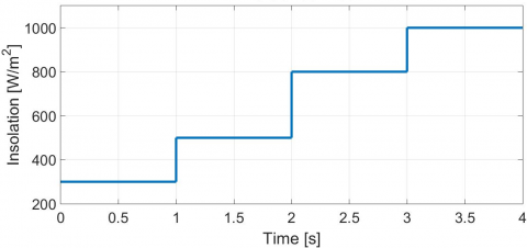
Figure 5. Variation of insolation
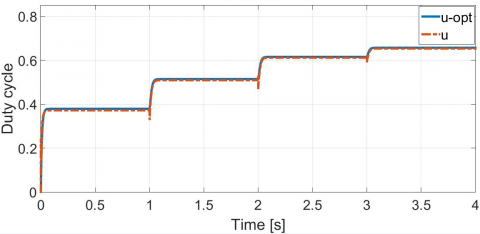
Figure 6. Curve of duty cycle
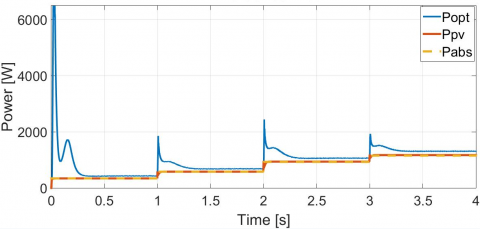
Figure 7. Power curves under variation of insolation
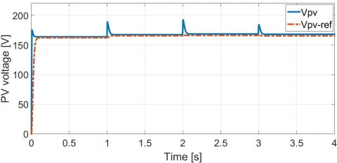
Figure 8. Curve of photovoltaic voltage
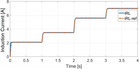
Figure 9. Curve of induction current
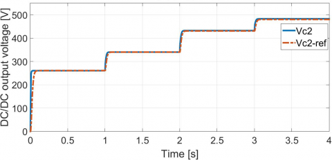
Figure 10. Curve of the boost converter’s output voltage
Figure 11. D-axis stator current curves comparison under variation of insolation
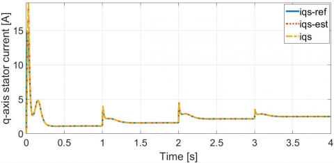
Figure 12. Q-axis stator current curves comparison under variation of insolation
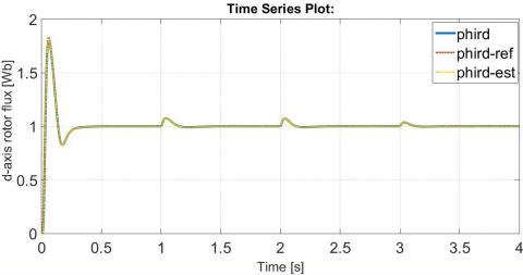
Figure 13. D-axis rotor flux curves comparison under variation of insolation
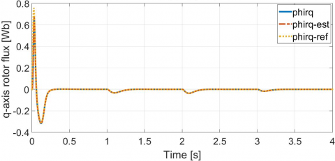
Figure 14. Q-axis rotor flux curves comparison under variation of insolation
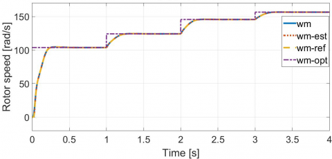
Figure 15. Rotor speed curves
The simulation test includes analyzing the controllers performance during both the transient and steady-state period. In this test, the insolation profile changes between 300W/m2 and 1000W/m2 in the Figure 5. The variations of the duty cycle, the PV power, the PV voltage, the inductance current end the load voltage, in response to the mentioned insolation changes are presented in Figures 6, 7, 8, 9 and 10.
As it is shown in the under figures, the different state variables of the PV conversion system, converge successively to their reference values i.e. the desired trajectory to track, with respect to the solar irradiation variation. The PV power and PV voltage curves show peaks during the transient mode, but despite that they present a very good convergence towards the reference curve in the steady-state period. Figures 11, 12, 13, 14 and 15 illustrate the response of the d-axis stator current, the q-axis stator current, the d-axis rotor flux, the q-axis rotor flux and the rotor speed, controlled by the second designed T-S fuzzy controller.
It is seen from these graphs, that the proposed T-S fuzzy control method presents a rapid convergence speed to the reference trajectory and consequently a good tracking accuracy is achieved. The d-axis rotor flux tracks the reference value, and hence the decoupling control characteristic between the rotor flux and the generator torque is assured. Likewise, the different upper curves show the evolution of the state variables and their estimated states delivered by the proposed T-S fuzzy observer under the changes of optimal rotor speed.
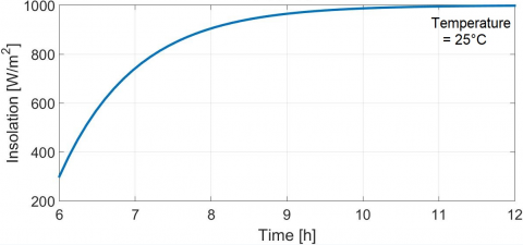
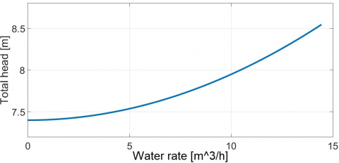
In the purpose of illustrating the characteristic of the pump H(Q), a continuous variation of the insolation is adopted in the Figure 16, starting from a minimum value of 200 W/m2 in 6h of the morning and finishing by a maximum value of 1000 W/m2 in 13h. The characteristic H(Q) is illustrated in the Figure 17.
Figure 16. Continuous variation of insolation
Figure 17. Characteristic of centrifugal pump H(Q)
In this paper a T-S fuzzy MPPT decentralized control method for Solar PV Powered Water Pumping System driven by Induction Motor was presented. Using the proposed MPPT T-S fuzzy controller for the first PV conversion system, this latter is forced to operate close to the MPP trajectory. While basing on the PV power delivered by the PVG, a reference motor speed value has been pre-calculated, in order to make the unit motor-pump operate in the maximum power conditions. The T-S fuzzy observer-based controller is developed for the IM. Furthermore, H∞ tracking performance is adopted, to ensure a disturbance rejection of abrupt climatic conditions variation. Controllers’ gains are obtained by solving sets of LMIs. The obtained simulation results show that the proposed T-S fuzzy approach exhibits a good tracking performance during transient and steady-state periods, likewise for both proposed T-S controllers, a fast convergence speed and an attenuation of disturbance effect due to rapidly changing climatic conditions by using a H∞ performance.
Future work will focus on the design of a Fault Tolerant Tracking Control (FTC) for the PV pumping system based on the IM. This control strategy will offsets the effect of the faults that can effect the speed sensor and will ensure the transfer of optimal power to unit motor–pump.
[1] Chunting, M., Correa, M.B.R., Pinto, J.O.P. (2010). The IEEE 2011 International Future Energy Challenge—Request for Proposals. In Proc. IFEC, pp. 1-24.
[2] Terki, A., Moussi, A., Betka, A., Terki, N. (2012). An improved efficiency of fuzzy logic control of PMBLDC for PV pumping system. Applied Mathematical Modelling, 36(3): 934-944. http://dx.doi.org/10.1016/j.apm.2011.07.042
[3] Betka, A., Moussi, A. (2004). Performance optimization of a photovoltaic induction motor pumping system. Renewable Energy, 29(14): 2167-2181. https://doi.org/10.1016/j.renene.2004.03.016
[4] Ellouze, M., Gamoudi, R., Mami, A. (2010). Sliding mode control applied to a photovoltaic water-pumping system. International Journal of Physical Sciences, 5(4): 334-344.
[5] Ameziane, M., Sefriti, B., Boumhidi, J., Slaoui, K. (2013). Neural network sliding mode control for a photovoltaic pumping system. Journal of Electrical Systems, 9(3).
[6] Lalouni, S., Rekioua, D., Rekioua, T., Matagne, E. (2009). Fuzzy logic control of stand-alone photovoltaic system with battery storage. Journal of power Sources, 193(2): 899-907. http://dx.doi.org/10.1016/j.jpowsour.2009.04.016
[7] Keating, L., Mayer, D., McCarthy, S., Wrixon, G.T. (1991). Concerted action on computer modeling & simulation. In Tenth EC Photovoltaic Solar Energy Conference, Springer, Dordrecht, pp. 1259-1265. http://dx.doi.org/10.1007/978-94-011-3622-8_317
[8] Chan, D.S.H., Phillips, J.R., Phang, J.C.H. (1986). A comparative study of extraction methods for solar cell model parameters. Solid-State Electronics, 29(3): 329-337. http://dx.doi.org/10.1016/0038-1101(86)90212-1
[9] Takagi, T., Sugeno, M. (1985). Fuzzy identification of systems and its applications to modeling and control. IEEE Transactions on Systems, Man, and Cybernetics, 1: 116-132. http://dx.doi.org/10.1109/TSMC.1985.6313399
[10] Tseng, C.S., Chen, B.S., Uang, H.J. (2001). Fuzzy tracking control design for nonlinear dynamic systems via T-S fuzzy model. IEEE Transactions on Fuzzy Systems, 9(3): 381-392. http://dx.doi.org/10.1109/91.928735
[11] Allouche, M., Dahech, K., Chaabane, M., Mehdi, D. (2018). Fuzzy observer-based control for maximum power-point tracking of a photovoltaic system. International Journal of Systems Science, 49(5): 1061-1073. http://dx.doi.org/10.1080/00207721.2018.1433246
[12] Kamwa, I., Grondin, R., Hébert, Y. (2001). Wide-area measurement based stabilizing control of large power systems-a decentralized/hierarchical approach. IEEE Transactions on Power Systems, 16(1): 136-153. http://dx.doi.org/10.1109/59.910791
[13] Hossain, M.J., Pota, H.R., Kumble, C. (2010). Decentralized robust static synchronous compensator control for wind farms to augment dynamic transfer capability. Journal of Renewable and Sustainable Energy, 2(2): 022701. http://dx.doi.org/10.1063/1.3336014
[14] Wang, Y., Guo, G., Hill, D.J. (1997). Robust decentralized nonlinear controller design for multimachine power systems. Automatica, 33(9): 1725-1733. http://dx.doi.org/10.1016/S0005-1098(97)00091-5
[15] Bian, T., Jiang, Y., Jiang, Z.P. (2014). Decentralized adaptive optimal control of large-scale systems with application to power systems. IEEE Transactions on Industrial Electronics, 62(4): 2439-2447. https://doi.org/10.1109/TIE.2014.2345343
[16] Jiang, Y., Jiang, Z.P. (2012). Robust adaptive dynamic programming for large-scale systems with an application to multimachine power systems. IEEE Transactions on Circuits and Systems II: Express Briefs, 59(10): 693-697. http://dx.doi.org/10.1109/TCSII.2012.2213353
[17] Marino, R., Tomei, P., Verrelli, C.M. (2005). A nonlinear tracking control for sensorless induction motors. Automatica, 41(6): 1071-1077. http://dx.doi.org/10.1016/j.automatica.2005.01.015
[18] Zina, H.B., Allouche, M., Souissi, M., Chaabane, M., Chrifi-Alaoui, L., Bouattour, M. (2018). A Takagi-Sugeno fuzzy control of induction motor drive: experimental results. International Journal of Automation and Control, 12(1): 44-61. http://dx.doi.org/10.1504/IJAAC.2018.088606
[19] Wang, W.J., Lin, W.W. (2005). Decentralized PDC for large-scale T-S fuzzy systems. IEEE Transactions on Fuzzy Systems, 13(6): 779-786. http://dx.doi.org/10.1109/TFUZZ.2005.859309
[20] Benlarbi, K., Mokrani, L., Nait-Said, M.S. (2004). A fuzzy global efficiency optimization of a photovoltaic water pumping system. Solar Energy, 77(2): 203-216. http://dx.doi.org/10.1016/j.solener.2004.03.025