Lav Kush Kumar* | Vijayshree Yadav | Joy Roy | Raja Ram Yadav
© 2022 IIETA. This article is published by IIETA and is licensed under the CC BY 4.0 license (http://creativecommons.org/licenses/by/4.0/).
OPEN ACCESS
In the present study, one-dimensional advection-dispersion equation with variable coefficients is solved numerically with help of PDEPE in a finite porous domain. The pollutant is entering from the left end of the domain along the direction of the flow. Two different types of groundwater velocities have been considered, one rapidly decreasing with position and time and the other one being of sinusoidal nature over position and time. The dispersion coefficient is taken proportional to the groundwater velocity. Transport is included the first order decay and zero-order production parameters being proportional to the exponentially decreasing function with position and time and also being of sinusoidal nature over position and time. The nature of pollutant and porous medium are considered chemically non-reactive. Initially, porous domain is considered not to be solute free. Numerical solutions are obtained for uniform and varying type point sources. In heterogeneous porous media, variations in the parameters of solute transport such as: seepage velocities, dispersion coefficients etc. can be easily deal through numerical models. The effects of various physical parameters on solute concentration profiles are illustrated graphically.
advection, dispersion, uniform and varying input, first-order decay, zero-order production, PDEPE
Nowadays, the groundwater locations lying in urban and rural areas are under the threat of excessive toxic chemicals reaching to domains because of industrial wastes and agriculture fertilizers and because of these geological formations lying beneath the earth surface and having very low groundwater velocity, the scientific study of solute transport in aquifer systems remains a challenging problem for hydrologists, environmental scientists and mathematicians. Mathematical models, those deal with one, two and three dimensional solute mixing and traversing are developed by drafting the real world problem into mathematical equations considering the geometry of domain, site of external source of solute and other relevant boundary conditions like fresh water recharge sites. These models provide solutions to ascertain current and to predict future level of solute concentration with time and position. The solute transport process and estimation of pollution levels in aquifer system can be understood through reliable mathematical models, but this is a difficult task in many circumstances. The geometrical structure of the aquifer system, properties of solute and groundwater velocity, etc are the major factors affecting solute transport process in aquifers. Unlike many of available literatures, in present problem dispersion and groundwater velocities are more generalized form and can take any feasible relation and may represent all the possible situations. Moreover, finite domain structure represents the real world situations far better in comparison to the semi-infinite. Solute transport in porous media is governed by second order parabolic partial differential equation known as advection-dispersion equation (ADE) which is solved numerically and obtained results are demonstrated with help of graphs. Several important analytical solutions in finite and infinite domains with different approaches for simulating the solute transport phenomena have been appeared in the published literature. Mathematical models are potential and efficient tools for understanding the behavior of pollutants in subsurface environments. Logan and Zlotnik [1] proposed an analytical solution with the decay term for periodic input conditions in a semi-infinite domain to overcome the fluctuations of the groundwater table. Barry and Sposito [2] derived an analytical solution of advection-dispersion equation with time-dependent transport dispersion coefficients. Kangle et al. [3] developed an analytical solution with scale dependent dispersion for solute transport in heterogeneous porous media. Yadav et al. [4] presented an analytical solution of one-dimensional advection-dispersion equation with unsteady flow in an adsorbing porous medium. Srinivasan and Clement [5, 6] developed analytical solutions with spatially varying initial condition and exponentially decaying source condition. Analytical solutions for one-dimensional solute transport problem with different point of view have been presented by many researchers in a semi-infinite or finite porous medium [7-11]. The majority of the analytical solutions of advection-dispersion equation are generally based on some ideal conditions, for example, using the assumptions on homogeneous porous medium, steady/unsteady velocity and uniform dispersion coefficients etc. [12-16].
In many real situations, the governing advection-diffusion equation is often non-linear, making it difficult to obtain analytical solutions. The numerical solution of advection-dispersion equation (ADE) plays an important role in finding approximate solution of the transport problem in aquifer systems. The numerical model becomes extremely useful especially when boundaries are complex or the coefficients are non-linear within the domain or both conditions occur simultaneously. The literature contains many numerical techniques for solving one-dimensional advection-dispersion equation problems. Tamora and Wadham [17] obtained a numerical solution of advection-dispersion equation for radial flow. Elfeki [18] developed a numerical model with the help of finite difference scheme to simulate the transient flow in the groundwater flow. Agusto and Bamingbola [19] studied numerical mathematical model for water pollution using implicit centered difference scheme for space and time. Pochai [20] obtained a hydrodynamic model and approximate solutions to the solvent-diffusion-reaction equation in a uniform reservoir. Gurarslan et al. [21] obtained numerical solution of advection-diffusion equation to estimate the pollutant in a river using finite difference schemes.
It is usually difficult to obtain an analytical solution of the advection-dispersion equation in which velocity and dispersion coefficient both vary with position and time hence the numerical solution is being obtained. Due to the complexity of traditional numerical methods, we present here the solution of advection-dispersion equation using PDEPE with different parameter values. The MATLAB PDE solver PDEPE solves initial-boundary value problems of parabolic and elliptic nature for systems of PDEs in one spatial variable x and time t. PDEPE uses an informal classification for the 1-D equations. PDEPE also solves certain 2-D and 3-D problems that reduce to 1-D problems due to angular symmetry. The heterogeneity of the porous medium plays a significant role on the solute transport. It causes variations in groundwater velocity [22, 23]. Considering this fact the seepage velocity is assumed to be exponential decreasing and sinusoidal nature with position and time variables. First order decay and zero-order production terms are also considered. Also dispersion coefficient is directly proportional to the groundwater velocity. The medium is supposed to be heterogeneous. The heterogeneity of the medium is because of slight variations in either distribution of porous or variation in pore size with position etc., in such a medium groundwater velocity, dispersion, etc. vary with position. This is a common feature of the aquifers and domain is considered of finite length in longitudinal direction that is along x-axis. Solutions are obtained for uniform and varying type input point sources. The input condition is assumed at a point other than the origin of the finite domain and second condition is considered at the end of the domain. Examples are included to illustrate the effect of time and spatial dependent dispersion coefficients on solute transport with the help of realistic input data taken from the published research literature.
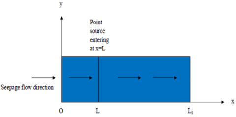
This study considers the solute transport problem for conservative solute in heterogeneous porous medium of finite length with a point source located at the point x=L of the domain of Figure 1. The one-dimensional mathematical expression of the advection-dispersion equation with first order decay and zero-order production may be written as [24, 25]:
$\frac{\partial C}{\partial t}=\frac{\partial}{\partial x}\left(D(x, t) \frac{\partial C}{\partial x}-u(x, t) C\right)-\gamma C+\mu$ (1)
where, $C\left[ ML ^{-3}\right]$ is the solute concentration in the liquid phase. $x[L], t[T]$ are position and time variable, respectively. $D\left[L^2 T^{-1}\right]$ and $u\left[ LT ^{-1}\right]$ are the solute dispersion coefficient and groundwater flow velocity, respectively. $\gamma\left[T^{-1}\right]$ and $\mu\left[ ML ^{-3} T ^{-1}\right]$ are the first order decay rate coefficient and zero-order production, respectively.
Figure 1. Schematic view of the proposed problem
2.1 Uniform continuous input point source condition
Let the pollutant enter into a heterogeneous finite porous domain at a fixed location x=L uniformly continuously along the flow in longitudinal direction. Groundwater flow is considered along the x-axis i.e. towards x=L to x=L1. The medium is assumed to be not solute free at initial time. It means some concentrations already exist before solute injection into the domain. Solute is continuously being entered to the aquifer. In many real situations the concentration of pollutants is maximum it begins to decrease with position and time when entering the aquifer.
Mathematically, initial and boundary conditions associated with Eq. (1) are as follows:
$C(x, t)=C_i \exp (-a x) ; t=0, L<x \leq L_1$, (2)
$C(x, t)=C_0 ; t>0, x=L$, (3)
$\frac{\partial C(x, t)}{\partial x}=\frac{u}{D} C ; t \geq 0 x=L_1$, (4)
Dispersion coefficient and groundwater velocity are taken as:
$\left.\begin{array}{l}u(x, t)=u_0 f(x, t) \\ D(x, t) \propto u(x, t) \Rightarrow D(x, t)=D_0 f(x, t) \\ \gamma(x, t)=\gamma_0 f(x, t) \\ \mu(x, t)=\mu_0 f(x, t)\end{array}\right\}$ (5)
where, $u_0, D_0, \gamma_0$ and $\mu_0$ are initial values of groundwater velocity, dispersion coefficient, first order decay and zero order production, respectively.
Here $f(x, t)$ is considered as a non-dimensional expression such that at $x=0$ or $t=0$ or both is zero then the value of $f(x, t)=1$. An implicit form of $f(x, t)$ is considered of two different forms as:
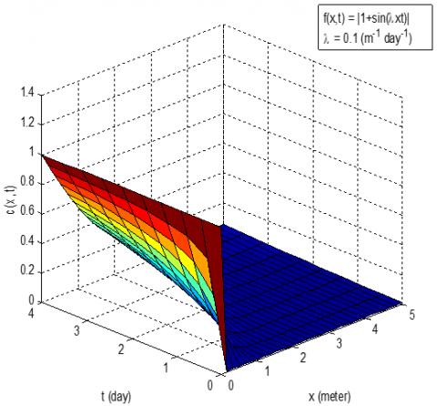
$\left.\begin{array}{l}(i) f(x, t)=\exp (-\lambda x t) \\ (i i) f(x, t)=|1+\sin (\lambda x t)|\end{array}\right\}$ (6)
Here, $\lambda\left[L^{-1} T^{-1}\right]$ represents a parameter whose dimension inverse of both position and time.
Substituting expressions from Eq. (5) in Eqns. (1-4), we have
$\frac{\partial C}{\partial t}=\frac{\partial}{\partial x}\left(D_0 f(x, t) \frac{\partial C}{\partial x}-u_0 f(x, t) C\right)-\left(\gamma_0 C-\mu_0\right) f(x, t)$ (7)
The initial and boundary conditions are
$C(x, t)=C_i \exp (-a x) ; t=0, L<x \leq L_1$ (8)
$C(x, t)=C_0 ; t>0, x=L$ (9)
$\frac{\partial C(x, t)}{\partial x}=\frac{u_0}{D_0} C ; t \geq 0, x=L_1$ (10)
2.2 Varying input point source condition
The source of input concentration may vary with time due to variety of reasons. This type of situation may also be described by a mixed type or third type condition and for all simulated scenarios, zero flux boundary condition is assumed along the longitudinal flow which is written as follows:
$-D \frac{\partial C(x, t)}{\partial x}+u C(x, t)=u_0 C_0\{1+\sin (m t)\}; t>0, x=L$ (11)
$\frac{\partial C(x, t)}{\partial x}=0 ; t \geq 0 x=L_1$ (12)
Using Eq. (5) in above boundary conditions Eqns. (11-12), we have
$\begin{aligned} &-D_0 f(x, t) \frac{\partial C}{\partial x}+ u_0 f(x, t) C = u_0 C_0\{1+\sin (m t)\} ; t>0, x=L\end{aligned}$ (13)
$\frac{\partial C(x, t)}{\partial x}=0 ; t \geq 0, x=L_1$ (14)
The solutions of the proposed problem for both the cases are obtained numerically with help of PDEPE through MATLAB and results are demonstrated graphically.
In order to demonstrate the concentration profiles with position and time, the advection-dispersion equation for finite domain $0 \leq x(m) \leq 5$ i.e. $L=0$ and $L_1=5$ is solved numerically using PDEPE through MATLAB and results are shown in Figures 2 - 9 for various physical parameters used in model. The values of common input parameters such as ground water velocity, dispersion coefficient, first order decay etc. are taken from published literature [26-29]. The concentration values are evaluated assuming reference concentration as $C_0=1.0, C_i=0.01$ in a finite domain along longitudinal direction. The medium is supposed to be heterogeneous. The units of position and time are considered in meter and day, respectively. The common input value are taken as: initial seepage velocity $u_0=0.12(meter/day)$, initial dispersion coefficient $D_0=0.20\left(\right.meter^2/day)$, heterogeneous parameter $m=0.01\left(day^{-1}\right)$, initial first order decay $\gamma_0=0.0020\left(\right.day\left.^{-1}\right)$, initial zero order production $\mu_0=0.0025\left( kg / meter ^3\right.day)$, time $t=4(day)$, a=0.015(meter-1) $\lambda=0.1\left(\right.meter^{-1}day\left.^{-1}\right)$. The concentration profiles have been demonstrated in the finite domain and the values of the physical parameters are given in each respective figure.
Case-I: Figures (2 & 3) are line graphs and (4 & 5) are surface graphs for the uniform input point source.
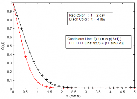
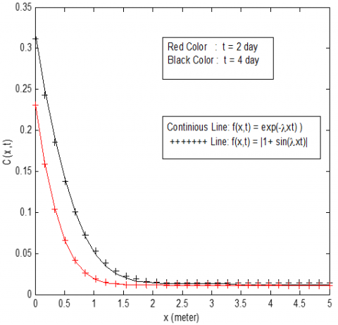
Figure 2. Concentration distribution from Eq. (7) for exponential decreasing and sinusoidal forms of velocity in uniform input at two different time
Figure 2 illustrates the concentration profiles for uniform continuous input point source at two different time for the solution in Eq. (7). Other effective parameters affecting the transport process within aquifer domain are common in each graph. The concentration level at a particular position in the domain decreases over time for both (sinusoidal and exponential) forms of velocity. The distribution of solute concentrations is nearly the same for both types of velocities, but the rehabilitation process in exponential form is occurring slightly faster than in sinusoidal. The concentration pattern increases with respect to time, whereas it decreases with respect to the position and after certain distance it becomes constant for all time. The solute concentration decreases gradually until it reaches to its steady state.
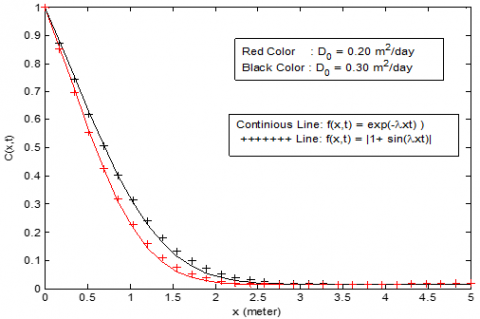
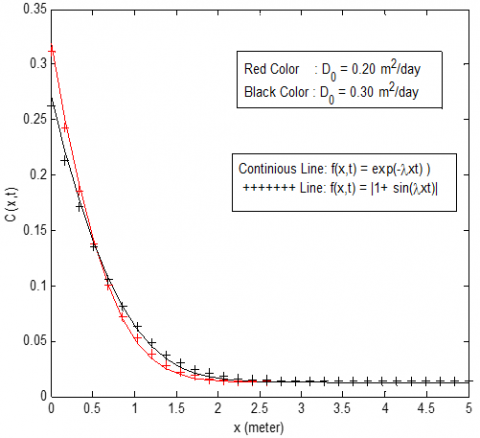
Figure 3. Concentration distribution from Eq. (7) for exponential decreasing and sinusoidal forms of velocity in uniform input at two different dispersion coefficient
Figure 3 demonstrates the dimensionless concentration distribution obtained by the solution of Eq. (7) at two different dispersion coefficients with other common input parameters in the uniform continuous input point source. At a particular position the concentration level is lower for a lower dispersion coefficient and higher for the higher dispersion coefficient in both forms of the velocity for exponential decreasing and the sinusoidal nature. The decreasing tendency of the concentration distribution with the position and the time is slightly faster in exponential decreasing nature than that in the sinusoidal nature. The contaminant concentration increases with respect to dispersion coefficient, whereas decreases with respect to the position and after certain distance it becomes steady. The patterns of solute concentrations are nearly the same for both forms of velocities.
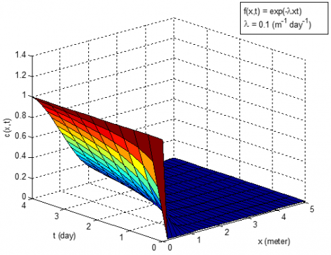
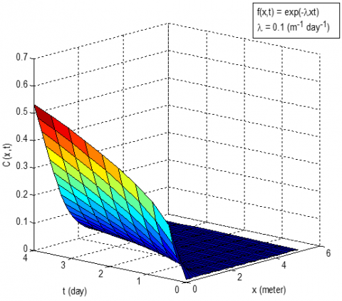
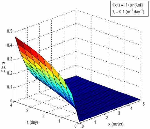
Figure 4. Concentration distribution from Eq. (7) for exponential decreasing form of velocity in the uniform type input
Figure 5. Concentration distribution from Eq. (7) for sinusoidal form of velocity in the uniform type input
Two surface graphs Figures 4 and 5 are drawn for the same set of data taking the exponential decreasing and sinusoidal form of velocity for the solution of Eq. (7) in the presence of uniform type input source. Concentration pattern decreases with respect to position and after certain distance it becomes steady. The decreasing tendency of contaminant concentration distribution with position and time is slightly faster in exponential nature than that in case of sinusoidal nature of velocity. The trends of concentration distribution are nearly similar in both forms (sinusoidal and exponential) of velocity.
Case-II: Figures 6 and 7 are line graphs and Figures 8 and 9 are surface graphs for the varying type input point source.
Figure 6 demonstrates the contaminant concentration profiles for varying nature input point source at two different time for the solution in Eq. (7) for exponential decreasing and sinusoidal nature of velocity. Contaminant concentration decreases with the increase of the position in both the case and finally tended to the stable value. The decreasing trend of concentration distribution with position and time is slightly faster in exponential nature than that in sinusoidal nature. At particular position the concentration level is lower for lower time and higher for higher time in both form of velocity for exponential decreasing and sinusoidal nature. The graph is the same for both types of input sources and a slight deviation can be seen between these two.
Figure 6. Concentration distribution from Eq. (7) for exponential decreasing and sinusoidal nature of velocity in varying type input at two different time
Figure 7. Concentration distribution from Eq. (7) for exponential decreasing and sinusoidal nature in varying type input at two different dispersion coefficient
Figure 7 represents the dimensionless concentration distribution predicted by the solution of Eq. (7) at two different dispersion coefficient assuming other parameters same as in previous figure. Concentration distribution attenuates with position and time. Near the boundary the contaminant concentration level is lower for higher dispersion coefficient and higher for lower dispersion coefficient in both form of velocity (exponential decreasing and sinusoidal nature). This view is reversing as moves away from the source boundary. The concentration distribution of solute concentrations is nearly the same for both forms of velocities, but the rehabilitation process in exponential form is occurring slightly faster than that in sinusoidal nature velocity.
Figures 8 and 9 demonstrate the dimensionless concentration distribution through surface graphs given by solution of Eq. (7) for varying input point source for exponential decreasing and sinusoidal nature of velocity, respectively. Contaminant concentration distribution attenuates with position and time in both the forms of velocities. The concentration distribution pattern decreases with respect to position and after a certain distance it becomes steady. The decreasing tendency of contaminant concentration distribution with position and time is slightly faster in exponential decreasing form of velocity than that in sinusoidal nature velocity. Initially at particular time concentration level is lower in sinusoidal nature than that in exponential nature. In both form of velocities, it is observed that at the other end of the porous domain the solute concentration values attain minimum and harmless concentration values.
Figure 8. Concentration distribution from Eq. (7) for exponential decreasing nature velocity in varying type input
Figure 9. Concentration distributions from Eq. (7) for sinusoidal nature velocity in varying type input
A numerical solution is developed for one-dimensional advection-dispersion equation in a one-dimensional finite heterogeneous porous domain with time and position varying dispersion coefficient and groundwater velocity by using PDEPE through MATLAB. Uniform continuous and varying nature input point source are the key feature of the study. Solute dispersion coefficient is taken directly proportional to groundwater velocity. This numerical result may be useful tool for identifying the level of solute concentration at any position and time. First order decay and zero order production terms are also taken as function of position and time. All parameters in the proposed model are taken dimensional here, and the contaminant concentration is obtained as a function of dimensional time and position. All position and time-dependent effective parameters affecting the concentrations distribution are shown with the help of graphs. Numerical solutions are considered more flexible than any analytical solution because they can handle complexities related to ideal situations such as heterogeneity of the medium: space, time varying dispersion parameters etc.
The authors are gratefully acknowledgement to Prof. Naveen Kumar, Ex-Dean Faculty of Science, B. H. U., Varanasi-India, for his valuable suggestions in improving the article.
[1] Logan, J.D., Zlotnik, V. (1995). The convection-diffusion equation with periodic boundary conditions. Applied Mathematics Letters, 8(3): 55-61. https://doi.org/10.1016/0893-9659(95)00030-t
[2] Barry, D.A., Sposito, G. (1989). Analytical solution of a convection-dispersion model with time-dependent transport coefficients. Water Resources Research, 25(12): 2407-2416. https://doi.org/10.1029/wr025i012p02407
[3] Kangle, H., van Genuchten, M.T., Renduo, Z. (1996). Exact solutions for one-dimensional transport with asymptotic scale-dependent dispersion. Applied Mathematical Modelling, 20(4): 298-308. https://doi.org/10.1016/0307-904X(95)00123-2
[4] Yadav, R.R., Vinda, R.R., Kumar, N. (1990). One-dimensional dispersion in unsteady flow in an adsorbing porous medium: An analytical solution. Hydrological Processes, 4(2): 189-196. https://doi.org/10.1002/hyp.3360040208
[5] Srinivasan, V., Clement, T.P. (2008). Analytical solutions for sequentially coupled one-dimensional reactive transport problems-Part I: Mathematical derivations. Advances in Water Resources, 31(2): 203-218. https://doi.org/10.1016/j.advwatres.2007.08.002
[6] Srinivasan, V., Clement, T.P. (2008). Analytical solutions for sequentially coupled one-dimensional reactive transport problems–Part II: Special cases, implementation and testing. Advances in Water Resources, 31(2): 219-232. https://doi.org/10.1016/j.advwatres.2007.08.001
[7] Yates, S.R. (1990). An analytical solution for one-dimensional transport in heterogeneous porous media. Water Resources Research, 26(10): 2331-2338. https://doi.org/10.1029/92WR01006
[8] Yates, S.R. (1992). An analytical solution for one-dimensional transport in porous media with an exponential dispersion function. Water Resources Research, 28: 2149-2154. https://doi.org/10.1029/WR026i010p02331
[9] Jaiswal, D.K., Kumar, A., Kumar, N., Yadav, R.R. (2009). Analytical solutions for temporally and spatially dependent solute dispersion of pulse type input concentration in one-dimensional semi-infinite media. Journal of Hydro-environment Research, 2(4): 254-263. https://doi.org/10.1016/j.jher.2009.01.003
[10] Jaiswal, D.K., Kumar, A., Yadav, R.R. (2011). Analytical solution to the one-dimensional advection-diffusion equation with temporally dependent coefficients. Journal of Water Resource and Protection, 3(1): 76-84. https://doi.org/10.4236/jwarp.2011.31009
[11] Yadav, R.R., Jaiswal, D.K. (2012). Two-dimensional solute transport for periodic flow in isotropic porous media: an analytical solution. Hydrological Processes, 26(22): 3425-3433. https://doi.org/10.1002/hyp.8398
[12] Rumer Jr, R.R. (1962). Longitudinal dispersion in steady and unsteady flow. Journal of the Hydraulics Division, 88(4): 147-172. https://doi.org/10.1061/JYCEAJ.0000740
[13] Kumar, N. (1983). Unsteady flow against dispersion in finite porous media. Journal of Hydrology, 63(3-4): 345-358. https://doi.org/10.1016/0022-1694(83)90050-1
[14] Chrysikopoulos, C.V., Sim, Y. (1996). One-dimensional virus transport in homogeneous porous media with time-dependent distribution coefficient. Journal of Hydrology, 185(1-4): 199-219. https://doi.org/10.1016/0022-1694(95)02990-7
[15] Kumar, N., Kumar, M. (1998). Solute dispersion along unsteady groundwater flow in a semi-infinite aquifer. Hydrology and Earth System Sciences, 2(1): 93-100. https://doi.org/10.5194/hess-2-93-1998
[16] Jaiswal, D.K., Yadav, R.R., Gulrana (2013). Solute-transport under fluctuating groundwater flow in homogeneous finite porous domain. Hydrogeol. Hydrol. Eng, 2(1). https://doi.org/10.4172/2325-9647.1000103
[17] Tamora J., Wadham, C. (2002). Numerical solution of advection-diffusion equations for radial flow. University of Oxford.
[18] Elfeki, A. (2003). Transient Groundwater Flow in Heterogeneous Geological Formations.(Dept. C). MEJ. Mansoura Engineering Journal, 28(1): 58-67. http://dx.doi.org/10.21608/bfemu.2021.140807
[19] Agusto, F.B., Bamigbola, O.M. (2007). Numerical treatment of the mathematical models for water pollution. Journal of Mathematics and Statistics, 3(4): 172-180. https://doi.org/10.3844/jmssp.2007.172.180
[20] Pochai, N. (2009). A numerical computation of a non-dimensional form of stream water quality model with hydrodynamic advection–dispersion–reaction equations. Nonlinear Analysis: Hybrid Systems, 3(4): 666-673. https://doi.org/10.1016/j.nahs.2009.06.003
[21] Gurarslan, G., Karahan, H., Alkaya, D., Sari, M., Yasar, M. (2013). Numerical solution of advection-diffusion equation using a sixth-order compact finite difference method. Mathematical Problems in Engineering, 2013: 672936. https://doi.org/10.1155/2013/672936
[22] Hassan, A.E., Cushman, J.H., Delleur, J.W. (1998). Significance of porosity variability to transport in heterogeneous porous media. Water Resources Research, 34(9): 2249-2259. https://doi.org/10.1029/98wr01470
[23] Simmons, C.T., Fenstemaker, T.R., Sharp Jr, J.M. (2001). Variable-density groundwater flow and solute transport in heterogeneous porous media: approaches, resolutions and future challenges. Journal of Contaminant Hydrology, 52(1-4): 245-275. https://doi.org/10.1016/s0169-7722(01)00160-7
[24] Freeze, R.A., Cherry, J.A. (1979). Groundwater, Prentice-Hall, Inc. Englewood Cliffs, New Jersey.
[25] Bear, J. (1972). Dynamics of Fluid in Porous Media. Elsvier Publ. Co. New York.
[26] Jaiswal, D.K., Kumar, A., Kumar, N., Singh, M.K. (2011). Solute transport along temporally and spatially dependent flows through horizontal semi-infinite media: dispersion proportional to square of velocity. Journal of Hydrologic Engineering, 16(3): 228-238. https://doi.org/10.1061/(ASCE)HE.1943-5584.0000312
[27] Singh, M.K., Ahamad, S., Singh, V.P. (2014). One-dimensional uniform and time varying solute dispersion along transient groundwater flow in a semi-infinite aquifer. Acta Geophysica, 62(4): 872-892. https://doi.org/10.2478/s11600-014-0208-7
[28] Bharati, V.K., Sanskrityayn, A., Kumar, N. (2015). Analytical solution of ADE with linear spatial dependence of dispersion coefficient and velocity using GITT. Journal of Groundwater Research, 3(4): 13-26.
[29] Kumar, A., Jaiswal, D.K., Kumar, N. (2010). Analytical solutions to one-dimensional advection–diffusion equation with variable coefficients in semi-infinite media. Journal of Hydrology, 380(3-4): 330-337. https://doi.org/10.1016/j.jhydrol.2009.11.008