Raja R. Yadav* | Joy Roy
OPEN ACCESS
In this paper, one-dimensional advection–diffusion equation for time and space dependent contaminant concentration in a homogeneous semi-infinite aquifer is solved numerically using Implicit Crank-Nicolson finite difference method. Dispersion and groundwater velocity are considered to have any mutually dependency and represented by some possible function of time. Initially, geological formation is supposed to be solute free. Input point source of continuous or discontinuous function of time is supposed to be acting along the flow at one end of the boundary. Flux type boundary condition is considered at infinity. The numerical solution is compared with the analytical solutions available in published literatures. The obtained result of the problem could be used as a new tool for the conception of complex situations in subsurface transport phenomenon which may not be solved analytically. The effects of parameters on the concentration dispersion are illustrated with the help of respective graphs.
advection, dispersion, aquifer, porous medium, crank-Nicolson method
Study of solute transport phenomena in porous medium has been a large area of interest of researchers. Solute transport in subsurface is usually described by the Advection-Dispersion Equation (ADE), which is derived by Fick’s law of diffusion and principle of conservation of mass. This equation includes various terms which account the physical procedure such as hydrodynamic dispersion, decay parameter, etc. Solute dispersion is a major phenomenon of solute transport in both saturated and unsaturated porous media [1].
In the modeling of groundwater flow and transport, the main issue is the hydraulic conductivity of the aquifers, which generally occurs at different aspects like porosity, permeability, dispersion and adsorption etc. Hydraulic conductivity depends on the geometry of aquifers. To predict the contaminant transport in the porous medium accurately and efficiently, many analytical / numerical solutions have been published in literatures for one, two and three-dimensional finite and semi-infinite porous formation. The semi-infinite porous medium usually represents the situation when the aquifer is quite large and other end of domain remains unaffected with input concentration in the time domain of study.
Solute in groundwater is moved by a variety of physical, chemical and biological processes [2]. Pickens and Grisak obtained a numerical model based on dispersivity vary temporally [3]. Later Jayawardena and Lui obtained a numerical solution with a time–dependent dispersion [4]. Zhou, Zhou and Selim obtained two methods for demonstrating the scale-dependent dispersivity [5, 6]. Dehghan developed numerical solution for the one-dimensional constant coefficient convection-diffusion equation [7]. Leij et al. attained solution using the Green’s function method with contaminant source as a boundary condition [8]. Jaiswal and Kumar presented analytical solution including the effect temporally dependent dispersion for varying input condition with constant velocity [9]. The movement of solute through the porous media is due to dispersion and advection phenomena. Dispersion may vary with time. Mathematically dependency represented with time function. Yadav and Roy proposed analytical solution of two-stages input source problem for space dependent dispersion and velocity [10]. Study of Mazaheri et al. involved several point sources with uniform dispersion and groundwater velocity in semi-infinite porous medium [11]. Kumar et al. also presented the solution for semi-infinite porous media along with time-dependent dispersion and velocity [12]. Das and Singh obtained solution for temporal dispersion and exponentially variable input in semi-infinite study [13]. Singh and Chatterjee studied for three dimensional flow with plane input source in a homogeneous semi-infinite porous media [14]. Study also dealt with two sub cases namely line and point source.
In order to deal the situations which may not be addressed with an analytical solution, numerical solution is sought for such problems. Numerical solutions are more flexible in comparison to analytical solutions. Wang H.F., Anderson M.P., and Woessner W.W. obtained analytical and numerical solutions with temporally dependent boundary conditions [15, 16]. Alam studied the influence of Dufour and Soret effects on free convection mass transfer over an inclined permeable stretching sheet in porous media and obtained numerical solution by using Rungu-kutte method with Nachtsheim-Swigert shooting iteration technique [17]. Numerical solutions are helpful in verifying analytical solutions. Jha and Yasuf obtained semi-analytical solution for time dependent flow in an annulus with partially filled porous material accounting due to sudden application of constant pressure gradient and verified it with implicit finite difference scheme [18].
Singh et al. presented numerical solution using explicit finite difference method [19]. Solution obtained by explicit finite difference methods depends upon stability factor. It may be observed concentration varies with selection grid size.
Singh et al. and Jaiswal et al. obtained the solution for time-dependent dispersion and groundwater velocity [19, 20]. The analytical solution is solved for dispersion directly proportional to groundwater velocity. Thus it is difficult to obtain analytical solution when the dependency is represented by ξ [21], where 1≤ξ≤2 and also the situations when input vary with large rate exponentially [19]. Moreover, Jaiswal et al. obtained analytical solution of periodic input and dispersion problem which is difficult or impossible to solve analytically for asymptotic or algebraic sigmoid or for any other temporal dispersion [20]. In the present paper, the governing partial differential equation for one-dimensional advection-dispersion equation is solved numerically by using Implicit Crank-Nicolson method which is unconditionally stable. The aquifer medium is assumed homogeneous, adsorbing and semi-infinite long. Dispersion and groundwater velocity are assumed to be either temporally dependent or constant and may have any feasible relationship and time dependency i.e. dispersion and groundwater velocity are generalized. This paper also deals with arbitrary input concentration of continuous/ discontinuous function of time. Hence generalization of temporal dispersion and groundwater velocity along with input source has broadened the application of this paper. Numerical solution has also been compared with published analytical solutions.
We considered the solute transport through a homogeneous semi-infinite aquifer. Initially, the domain is assumed to be free from solute, it means that domain contains no contamination. Solute movement is considered along the flow in the medium and dispersion coefficient, groundwater velocity is either constant or any bounded function of time in the time domain [0, ∞]. The contaminant is injected along the flow through left boundary i.e. x=0. Input concentration may be any continuous or discontinuous and pulse type function of time. The inlet conditions of the flow system are assumed temporally dependent. The one-dimensional advection–dispersion equation which is a parabolic second order partial differential equation derived from Darcy’s law and conservation of mass [22].
$R \frac{\partial c^{\prime}}{\partial t^{\prime}}=\frac{\partial}{\partial x^{\prime}}\left(D\left(x^{\prime}, t^{\prime}\right) \frac{\partial c^{\prime}}{\partial x^{\prime}}-u(x, t) c^{\prime}\right)$ (1)
c’[ML-3] the solute concentration of the pollutant, x’[L] and time t’[T]. D[L2T-1] and u[LT-1] are the longitudinal dispersion and groundwater velocity respectively. R is retardation factor which is a dimensionless quantity. First term on the left and the right-hand side the Eq. (1) describes change in concentration with time in liquid phase and the influence of the dispersion on the concentration distribution in longitudinal direction respectively while second term on the right-hand side represents the change of concentration due to advective transport in longitudinal direction. In reality, hydraulic gradient accounts for changes in velocity and dispersion coefficient in the aquifer. The present article is compatible with all the possible relation in dispersion and groundwater velocity. Some of those are described as:
Since dispersion and seepage velocity are assumed to be either constant or time dependent. Let D(x,t)=D0f1(n’t’) and u(x,t)=u0f2(n’t’), where D0[L2T-1],u0[LT-1] are constants and f1(n’t’)(≥0),f2(n’t’)(≥0) are any function time that provide feasible relation between dispersion and groundwater velocity and n’[T-1] is a unsteady parameter and we have chosen f1(n’t’) and f2(n’t’) such that these are never unbounded and discontinuous for a finite time and represent dispersion and groundwater velocity. It is obvious that if f1(n’t’)=1 and f2(n’t’)=1 then dispersion and flow velocity reduce to constant. The Eq. (1) may be written as:
$R\frac{\partial c'}{\partial t'}=\frac{\partial }{\partial x'}\left( {{D}_{0}}{{f}_{1}}(n't')\frac{\partial c'}{\partial t'}\text{-}{{u}_{0}}{{f}_{2}}(n't')c' \right)$ (2)
Initially i.e. at time, it is assumed that there is no concentration present in the domain. At one end of the domain slolute is injected along the flow that may be represented mathematically by some function of time. In present paper the input may be any continuous/discontinuous bounded function of time. Concentration gradient is assumed zero at infinity that is another end of the semi-infinite domain. Mathematically initial and boundary condition may be written as:
C’(x’,t’)=0; t’=0, x’ ≥0 (3)
C’(x’,t’)=c0f(m’t’);0<t’,x’=0 (4)
$\frac{\partial c'(x',t')}{\partial x'}=0;as\text{ x }\!\!'\!\!\text{ }\to \infty \text{,t }\!\!'\!\!\text{ }\ge \text{0}$ (5)
where, c0[ML-3] is the reference concentration and m’[T-1] is an unsteady parameter.f(m’t’) represents any continuous or discontinuous function of time. The Analytical solution of advection-dispersion equation (2) with generalize input source boundary conditions (3-5) along with generalize temporal dispersion and groundwater velocity is almost impossible to solve analytically.
The implicit Crank-Nicolson finite difference method is used to obtain the solution. Using following parameters in non-dimensional form [19];
$c=\frac{c'}{{{c}_{0}}};x=\frac{x'{{u}_{0}}}{{{D}_{0}}};t=\frac{t'u_{0}^{2}}{{{D}_{0}}};m=\frac{m'{{D}_{0}}}{u_{0}^{2}};n=\frac{n'{{D}_{0}}}{u_{0}^{2}}$ (6)
Using equation (6), Eq. (2) and Eqns. (3-5) reduced into non-dimensional form as:
$R\frac{\partial c}{\partial t}={{f}_{1}}(nt)\frac{{{\partial }^{2}}c}{\partial {{x}_{2}}}-{{f}_{2}}(nt)\frac{\partial c}{\partial x}$ (7)
C(x,t)=0; t=0, x≥0 (8)
C(c,t)=f(mt); 0<t, x=0 (9)
$\frac{\partial c(x,t)}{\partial x}=0;as\text{ x}\to \infty \text{,t}\ge \text{0}$ (10)
Applying Crank-Nicolson implicit finite difference method on Eqns. (7-10) may be expressed [25]
$R\frac{{{c}_{i,j}}+1-{{c}_{i,j}}}{\Delta t}=\left\{ \frac{{{f}_{1}}(n.j.\Delta t)+{{f}_{1}}(n.(j+1).\Delta t)}{2} \right\}\times \frac{{{c}_{i-1,j}}-2{{c}_{i,j}}+{{c}_{i+1,j}}+{{c}_{i-1,j+1}}-2{{c}_{i,j+1}}+{{c}_{i+1,j+1}}}{2{{(\Delta x)}^{2}}}-\left\{ \frac{{{f}_{2}}(n.j.\Delta t)+{{f}_{2}}(n.(j+1).\Delta t)}{2} \right\}$
$\frac{{{c}_{i+1,j+1}}-{{c}_{i-1,j+1}}+{{c}_{i+1,j}}-{{c}_{i-1,j}}}{4\Delta \text{x}}$ (11)
Corresponding initial and boundary conditions may be written as:
$c(0,j)=f(m.\Delta t.j);\forall i$ (12)
$c(0,j)=f(m.\Delta t.j);\forall j$(13)
$\frac{{{c}_{i+1,j}}-{{c}_{i,j}}}{\Delta x}=0;i\to \infty $(14)
where, index i refers to x and j refers to t, △x=xi+1-xi and△t=ti+1-ti.If the value concentration at time is known then value of the concentration at time t+△t may be evaluated. We substitute i=1,2,2,…,N-1 where corresponds to∞. Eq. (11) gives tri-diagonal system of equation with initial and boundary conditions. Eqns. (11-14), which is solved with help of Thomas algorithm [26]. Implicit Crank-Nicolson Method finite difference method is a second order method in time and proposes no restrictions in space and time and which is unconditionally stable. In order to compute the space and time steps are taken as △x=0.01 and △t=0.0001.
The present article is flexible to deal any relation between dispersion and groundwater velocity and any temporal nature point input source acting along the flow in a homogeneous porous media. Utility of this article can be understood with help of three following numerical examples named. The numerical solutions for the present problem are computed for the given set of input as; c0=1.0, ci=0.0 and R=1.15. The graphical representations are anticipated in the finite length of the domain 0≤x’(km) ≤5 along longitudinal flow direction for different input source contaminants. The geological formation is supposed to be homogeneous. The values for groundwater velocity and dispersion coefficient are taken respectively u0(km year-1)=0.01 and D0(km2year-1)=0.1. The numerical solutions are obtained through Implicit Crank Nickolsan method described above and the particular cases are discussed and illustrated for a set chosen set of data either taken from published literatures or empirical relationship. For example, the range of groundwater velocity, keeping in view the different types of soils of aquifer lies between 2 m/day to 2 m/year [27].
4.1 Numerical examples 1
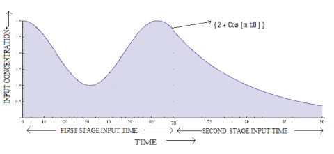
The contamination introduction into one end of water body is supposed to be of two stages and it is assumed that contaminant is some sinusoidal in nature in first stage and then starts decreasing exponentially from there [20]. It can be related to real life situation by supposing that the industrial contaminant injection remains sinusoidal in nature up to some year and then starts decreasing from there under some rehabilitation process. Groundwater velocity is asymptotic function of time and dispersion is some exponent ξto groundwater velocity i.e. D∝uξi.e., dispersion, groundwater velocity and input may be represented as:
$u=u_{0}\left\{m^{\prime} t^{\prime} /\left(m^{\prime} t^{\prime}+k\right)\right\}$ and $D=D_{0}\left\{m^{\prime} t^{\prime} /\left(m^{\prime} t^{\prime}+k\right)\right\}^{\xi}$
$f\left(m^{\prime} t^{\prime}\right)=\left\{\begin{array}{l}{2+\cos \left(m^{\prime} t^{\prime}\right) ; 0<t^{\prime} \leq t_{0}^{\prime}} \\ {\left\{2+\cos \left(m^{\prime} t_{0}^{\prime}\right)\right\} \exp \left[-\lambda^{\prime}\left(t^{\prime}-t_{0}^{\prime}\right)\right] ; t_{0}^{\prime}<t^{\prime}}\end{array}\right.$
Figure 1. Schematic diagram of input source with time injected at x=0 (km)
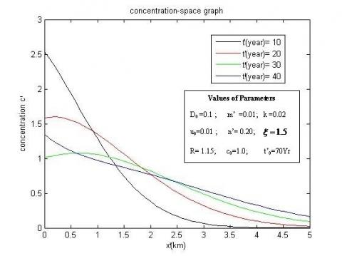
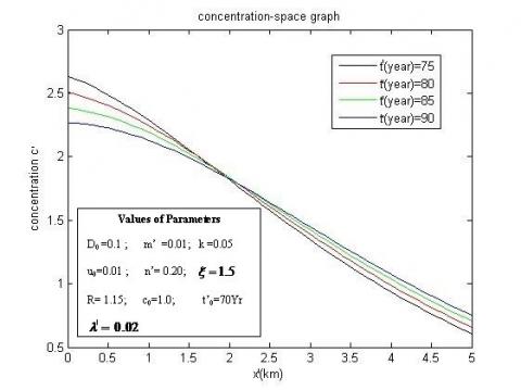
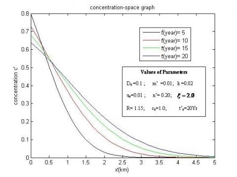
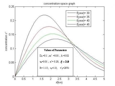
The figure 1 represents the graphical representation of the input concentration with time. In figure 2 the concentration fluctuation at x'(km)=0 is due to sinusoidal input in the first stage. It may be noticed that concentration distributes along the domain. Figure 3 is drawn for second stage input in which concentration reduces exponentially with time. At x'(km)=0 concentration is dropping gradually is due to decreasing input concentration. Atx'(km)=5 concentration increases it suggests concentration moving away from the source.
Figure 2. Concentration distribution in first stage input for various times
Figure 3. Concentration distribution in second stage input for various times
4.2 Numerical example 2
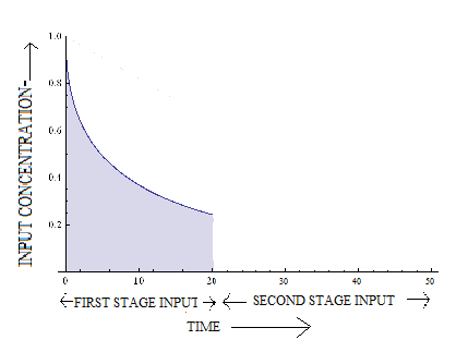
Solute transport depends upon the flow, nature of the solute, geometry of the medium and time duration. But at a point of an aquifer the pollutants reach due to percolation from a point source taking place on the surface. It means if source stops functioning at sudden, the contaminant remains present in domain and spreads in it. Such input is termed as pulse type.
Groundwater velocity is sinusoidal function of time [19] and dispersion is some exponent to groundwater velocity i.e. $D∝u^ξ$ i.e., dispersion, groundwater velocity and input may be represented as:
$u=u_{0}\left\{1-\sin \left(k m^{\prime} t^{\prime}\right)\right\}$ and $D=D_{0}\left\{1-\sin \left(k m^{\prime} t^{\prime}\right)\right\}^{\xi}$
$f\left(m^{\prime} t^{\prime}\right)=\left\{\begin{array}{l}{\exp \left(-\sqrt{m^{\prime} t^{\prime}}\right) ; 0<t^{\prime} \leq t_{0}^{\prime}} \\ {0 ; t>t_{0}^{\prime}}\end{array}\right.$
Figure 4. Schematic diagram of input source with time injected at x=0 (km)
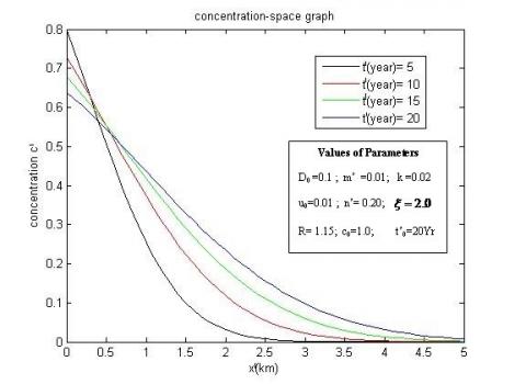
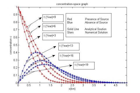
Figure 5. Concentration distribution in presence of input for various times
Figure 6. Concentration distributions in absence of input for various times
The figure 4 demonstrates graphical representation of the input concentration with time that concentration is exponentially decreasing in first stage and suddenly injected concentration is absent in second stage. In figure 5 the concentration decreases with time at x'(km)=0. This because exponentially decreasing input in the first stage. It may be noticed that concentration propagates along the domain due to advection and also disperses in the domain. Figure 6 is drawn for second stage input in which no concentration in injected i.e. source concentration is assumed absent at x'(km)=0. Due to absence of source, the concentration x'(km)=0 at is zero and already injected concentration gradually disperses and travels with the flow.
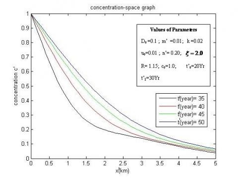
4.3 Numerical example 3
In this application, the contamination injection is supposed to be of three stages it assumed that contaminant release is exponential in nature in first stage and zero in second stage then constant from there in third stage. Groundwater velocity is algebraic sigmoid function of time [19] and dispersion is some exponent to groundwater velocity i.e. $D∝u^ξ$ i.e., dispersion and groundwater velocity and input may be represented as:
$u=u_{0}\left\{m^{\prime} t^{\prime} / \sqrt{\left(m^{\prime} t^{\prime}\right)^{2}+k^{2}}\right\} \qquad$ and $\quad D=D_{0}\left\{m^{\prime} t^{\prime} /\right.$
$\sqrt{\left(m^{\prime} t^{\prime}\right)^{2}+k^{2}} \}^{\xi}$
$f\left(m^{\prime} t^{\prime}\right)=\left\{\begin{array}{l}{\exp \left(-\sqrt{m^{\prime} t^{\prime}}\right) ; 0<t^{\prime} \leq t_{0}^{\prime}} \\ {0 ; t_{0}^{\prime}<t \leq t_{1}^{\prime}} \\ {1 ; t^{\prime}>t_{1}^{\prime}}\end{array}\right.$
Figure 7. Schematic diagram of input source with time injected at x=0 (km)
Figure 8. Concentration distribution at first stage input for various times
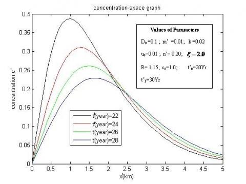
Figure 9. Concentration distribution at second stage input for various times
Figure 10. Concentration distribution at third stage input for various times
The Figure 7 is a schematic representation of input nature. The three stages source, namely exponential decreasing in first, absent of source in second and lastly a constant input. Figure 8 indicates that the concentration decreases with time at x'(km)=0. The input concentrations, at the origin, are different at each time. It attenuates with position and time. Figure 9 illustrates the concentration profiles once the source of the pollution is eliminated, i.e., the input concentration remains zero in the time domain. The concentration at origin i.e. at x'(km)=0 is zero because source is eliminated but already existing contaminant spreads away in the region. The solute concentration behaviour of constant input concentration of the third stage is shown in figure 10. This figure reveals that concentration value at x'(km)=0 is constant. Concentration at some point space is due to input of concentration at all three stages. It recorded that concentration near the source first decreases exponentially then reduces to minimal at absence of source and then increases in last stage.
All these three examples those represent three solute transport problem may be difficult or impossible to solve analytically.
The present numerical solution is verified with the two existing analytical solution. These follows as;
5.1 Verification 1
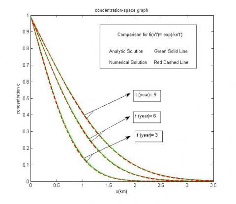
The numerical solution is verified by available literature [19]. For this purpose, the first order decay, zero order production and initial concentration are assumed to be zero in article [19] .The data set that was used for this validation is same as the one used for conducting this present article with $f\left(m^{\prime} t^{\prime}\right)=c_{0} \exp \left(-m^{\prime} t^{\prime}\right)$. The value of the parameters are considered as, dispersion coefficient $D_{0}\left(k m^{2} y e a r^{-1}\right)=0.1$; Seepage velocity $u_{0}\left(k m \cdot y e a r^{-1}\right)=0.01$;$m^{\prime}\left(y e a r^{-1}\right)=0.001$; Reference concentrations c0=1.0, ci=0.0
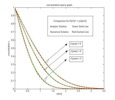
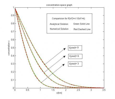
. The retardation factor is 1.29722 using $R=1+\frac{\rho}{K_{d}}\left(\frac{1-n_{p}}{n_{p}}\right)$ [19] where for clay np=0.55 density $\rho=999$ and $K_{d}=\frac{K_{1}}{K_{2}}$ with $K_{1}=0.000004$ and $K_{2}=0.02$. In Singh et al., the dispersion is directly proportional to groundwater velocity and groundwater velocity is time dependent [19]. Therefore, in present article $D(x, t) \propto u(x, t) \quad$ i.e. $\quad f_{1}\left(n^{\prime} t^{\prime}\right)=f_{2}\left(n^{\prime} t^{\prime}\right)$. The concentration pattern is obtained for different temporal functions of velocity Singh et al. (2015) namely exponentially decreasing function, asymptotic function, sinusoidal function and algebraic function [19]. The comparison between present article numerical solution and analytical solution [19] is done in following figures (11-14) for above mentioned temporal velocities. In following Figures the ‘Analytical Solution’ and ‘Numerical Solution’ refers for Singh et al. and present article, respectively [19].Figure 11. Comparison of contaminant concentration for numerical and analytical solution at different times for velocity defined as exponential decreasing function of time
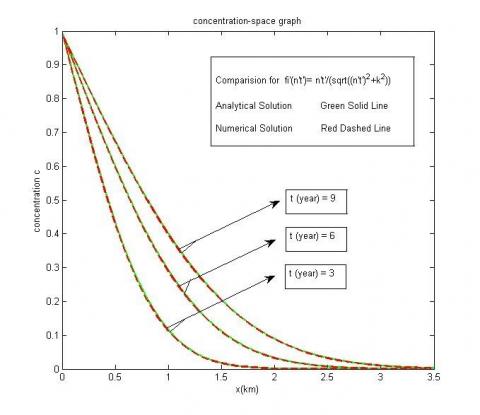
Figure 11, 12, 13 and 14 illustrates the comparison of the results obtained from the present numerical model with that obtained by Singh et al. [19]. All the figures exhibit excellent agreement between analytical solution and numerical solution of present article solution. A perfect agreement may be observed between the results obtained by Singh et al. [19].
Figure 12. Comparison of contaminant concentration for numerical and analytical solution at different times for velocity defined as sinusoidal function of time
Figure 13. Comparison of contaminant concentration for numerical and analytical solution at different times for velocity defined as algebraic sigmoid function of time
Figure 14. Comparison of contaminant concentration for numerical and analytical solution at different times for velocity defined as asymptotic function of time
5.2 Verification 2
Numerical solution obtained for uniform pulse type input is compared with analytical solution obtained by Kumar et al. [12]. Input data are takes as follows:
$f\left(m^{\prime} t^{\prime}\right)=\left\{\begin{array}{l}{c_{0}; 0<t \leq t_{0}} \\ {x=0} \\ {0 ; t>t_{0}}\end{array}\right.$
The value of the parameters are considered as, dispersion coefficient $D_{0}\left(k m^{2} y e a r^{-1}\right)=0.1$; groundwater velocity $u_{0}\left(k m^{-} y e a r^{-1}\right)=0.01$; concentrations c0=1.0, ci=0.0
(kumar et al. [12]); The retardation factor R=1.15; n'=0.04; with zero first order decay and zero order production in kumar et al. [12]. The dispersion is directly proportional to groundwater velocity and groundwater velocity is time dependent i.e. $D^{\prime}(x, t) \propto u^{\prime}(x, t)$ and $\quad f_{1}\left(n^{\prime} t^{\prime}\right)=f_{2}\left(n^{\prime} t^{\prime}\right)=\exp \left(-n^{\prime} t\right)$. The time of elimination of source is t0(year)=10. The following figure 15 shows the comparison between the numerical and analytical solution..Figure 15. Comparison between analytical and numerical solution for different times
Figure 15 shows a good agreement in analytical solution and numerical results. From a remediation perspective, the numerical solution is a more convenient tool for providing better and useful information in designing risk assessments and clean-up systems in subsurface water table.
This paper presents numerical solution for one-dimensional advection dispersion equation with a constant and time dependent dispersion coefficient for conservative solute transport in semi-infinite domain. The dispersion coefficient is assumed either constant or temporally dependent. The dispersion is taken as an exponent seepage velocity. The input source concentration is assumed any generalized function of time. Effect of dispersion coefficient, retardation factor and seepage velocity on solute concentration profiles has been discussed and demonstrated graphically. Majority analytical solutions fail to furnish satisfactory results in the case of complex boundary conditions for homogeneous porous formations. In such cases, numerical solutions will furnish a better substitute to the modelling of contaminant transport through aquifer. The derived model results have been verified by comparing these to the published analytical solutions and were found to be in good agreement with available analytical solutions.
c' concentration of the solute, kg m-3
c dimensionless concentration of solute
D longitudinal dispersion coefficient, m2s-1
u unsteady groundwater velocity, ms-1
D0 initial dispersion coefficient dispersion, m2s-1
u0 initial groundwater velocity, ms-1
c0 reference / source concentration
x' distance measured origin, m
x dimensionless distance measured origin
t' time, s
t dimensionless time
m' unsteady parameter regulates input, s-1
m dimensionless unsteady parameter
n' unsteady parameter regulates dispersion, s-1
n dimensionless unsteady parameter
λ' unsteady parameter regulates input, s-1
R dimensionless retardation factor
ξ dimensionless parameter establishes relation
between dispersion and groundwater
△x grid size of space variable
△t grid size of time variable
np porosity of geological formationξ
K dimensionless constant
Kd distribution coefficient
K1 adsorbing coefficient in solid
K2 adsorbing coefficient in liquid
[1] Lewis J, Sjostrom J. (2010). Optimizing the experimental design or soil columns in saturated and unsaturated transport experiments. Contaminant Hydrology 115: 1-4. https://doi.org/10.1016/j.jconhyd.2010.04.001
[2] Nielsen DRM, Van Genuchten MTh, Biggar JW. (1986). Water flow and solute transport processes in the unsaturated zone. Water Resour. Res. 22(95): 89S-108S. https://doi.org/10.1029/WR022i09Sp0089S
[3] Pickens JF, Grisak GE. (1981). Modeling of scale dependent dispersion in a hydrogeologic systems. Water Resour. Res. 17(6): 1701-1711. https://doi.org/10.1029/WR017i006p01701
[4] Jayawardena AA, Lui PH. (1984). Numerical solution of the dispersion equation using a variable dispersion coefficient: Method and applications. Hydrol. Sci.J. 29(3): 293–309. https://doi.org/10.1080/02626668409490947
[5] Zhou L. (2002). Solute transport in layered and heterogeneous soils. PhD dissertation, Louisiana State University, Baton Rouge, Louisiana, USA.
[6] Zhou LZ, Selim HM. (2002). A conceptual fractal model for describing time-dependent dispersivity. Soil Sci. 167(3): 173–183. https://doi.org/10.1097/00010694-200203000-00002
[7] Dehghan M. (2005). On the numerical solution of the one-dimensional convection-diffusion equation. Mathl Probl Eng. 1: 61-74. https://dx.doi.org/10.1155/MPE.2005.61
[8] Leij FJ, Priesack E, Schaap MG. (2000). Solute transport modeled with Green’s functions with application to persistent solute sources. J. Contami. Hydrol. 41: 155-173. https://doi.org/10.1016/S0169-7722(99)00062-5
[9] Jaiswal DK, Kumar A. (2011). Analytical solutions of advection-dispersion equation for varying pulse type input point source in one-dimension. International Journal of Engineering, Science and Technology 3(1): 22-29. https://doi.org/10.4314/ijest.v3i1.67636
[10] Yadav RR, Roy J. (2018). Solute transport phenomena in a heterogeneous semi-infinite porous media: an analytical solution. Int. J. Appl. Comput. Math 4: 135. https://doi.org/10.1007/s40819-018-0567-x
[11] Mazaheri M, Samani JMV, Samani HMV. (2013). Analytical solution to one-dimensional advection-diffusion equation with several point sources through arbitrary time-dependent emission rate patterns. J. Agr. Sci. Tech. 15: 1231-1245.
[12] Kumar A, Jaiswal DK, Yadav RR. (2011). One-dimensional solute transport for uniform and varying pulse type input point source with temporally dependent coefficients in longitudinal semi-infinite homogeneous porous domain. International Journal of Mathematics and Scientific Computing 1(2): 56-66.
[13] Das P, Singh MK. (2014). Solute dispersion with linear isotherm in unsteady groundwater flow in semi-infinite aquifer. International Conference on Modeling and Simulation of Diffusive Process and Applications (ICMSDPA), pp. 60-67.
[14] Singh MK, Chatterjee A. (2016). Solute dispersion in a semi-infinite aquifer with specified concentration along an arbitrary plane source. Journal of Hydrology 541: 928-934. https://doi.org/10.1016/j.jhydrol.2016.08.003
[15] Wang HF, Anderson MP. (1982). Introduction to groundwater modelling, finite difference and finite element methods. Academic Press.
[16] Anderson MP, Woessner WW. (1992). Applied groundwater modeling—simulation of flow and advective transport. Academic Press, Inc., San Diego, CA, p. 381.
[17] Alam Md. S. (2016). Mathematical modeling for the effects of thermophoresis and heat generation/ absorption on MHD convective flow along the inclined stretching sheet in presence of Dufour sorret effect. Mathematical Modelling of Engineering Problems 3(3): 119-128. https://doi:10.18280/mmep.030302
[18] Jha BK, Yasuf TS. (2018). Transient pressure driven flow in an annulus partially filled with porous material: Azimuthal pressure gradient. Mathematical Modelling of Engineering Problems 5(3): 260-267. https://doi.org/10.18280/mmep.050320
[19] Singh MK, Das P, Singh VP. (2015). Solute transport in a semi-infinite geological formation with variable porosity. J. Engineering Mechanics, ASCE 141(11). https://doi.org/10.1061/(ASCE)EM.1943-7889.0000948
[20] Jaiswal DK, Yadav RR, Gulrana. (2013). Solute-transport under fluctuating groundwater flow in homogeneous finite porous domain. J. Hydrogeol Hydrol Eng. 2(1). https://doi.org/10.4172/2325-9647.1000103
[21] Freeze RA, Cherry JA. (1979). Groundwater, Prentice-Hall. Englewood Cliffs, NJ.
[22] Bear J. (1972). Dynamics of Fluid in Porous Media. Elsevier Publication Co. New York.
[23] Yim CS, Mohsen MFN. (1992). Simulation of tidal effects on contaminant transport in porous media. Ground Water 30(1): 78-86. https://doi.org/10.1111/j.1745-6584.1992.tb00814.x
[24] Scheidegger AE. (1957). The physics of flow through porous media. University of Toronto Press, Toronto, 329.
[25] Shukla AK, Pandya N. (2016). Effects of thermophoresis, Dufour, hall and radiation on an unsteady MHD flow past an inclined plate with viscous dissipation, chemical reaction and heat absorption and generation. Journal of Applied Fluid Mechanics 9(1): 475-485.
[26] Brice Carnahan HL, Wilkes JO. (1969). Applied Numerical Methods. John Wiley and Sons, New York.
[27] Todd DK. (1980). Groundwater Hydrology. John Wiley, New York, USA.