R. Senthil Kumaran | G. Nagarajan
OPEN ACCESS
In this paper, the performance of hierarchical routing and fault tolerant routing scheme are combined and proposed a protocol named Hierarchical Energy Balanced Fault Tolerant Multipath Routing (HEBFTMR). Due to the hierarchical scheme adopted, cluster head energy level is saved. Cluster head in lower region can communicate to the higher region cluster head via the intermediate level cluster heads. Cluster head is changed frequently to equalize the load among the cluster members in the cluster. This cluster head is selected based on the following factors: residual energy, node weightage, distance between the neighbour nodes and the distance between the neighbour node and base station. Multipath routing is established to transmit data from the member node to the cluster head node for efficient data transmission. This is necessary due to the nature of sensors has frequent link broken. If the link is broken, neighbour node selection is important to route the data efficiently. The tolerant energy level of the sensor for route the data is determined. When the energy level decreases below the threshold value, other neighbour node is selected. Simulation results reveal that the proposed scheme proves that this combined scheme performs well when compared to the existing scheme in WSN environment.
clustering, energy efficiency, fault tolerant neighbour node, hierarchical routing
WSN is the recent technology which consist of several advantages like infrastructure less topology, less cost, mobility environment and depends on application specific Sensor nodes consume energy for transmitting, receiving and also for routing the sensed data from one position to other position (node). Energy is the most important factor in wireless sensor networks. Network lifetime depends on the energy of the sensors in the field / environment. The energy saving issue has augmented the importance of network lifetime and thus becomes the major research area for the growth in wireless sensor network applications. The proposed protocol utilizes proper balancing the load of the clusters to save the energy of the sensors and also establishes a multipath fault tolerant network for efficient routing. To achieve this proper balancing, periodical clustering is attempted. This shortens the network lifetime. This can be overcome by uniform sized partitioning of the network and also uses multipath routing scheme for proper routing. Also, hierarchical routing is implemented to decrease the overall energy consumption to improve network lifetime. Generally, the periodic rotation of cluster head may improve the network lifetime when the network is equally distributed. Hence, the selection of cluster head plays a major role in wireless sensor networks. The proposed technique called Hierarchical Energy Balanced Fault Tolerant Multipath Routing (HEBFTMR) Protocol is presented to save the energy level of the sensor and utilizes proper routing leads to improve the sensor lifetime.
Sajjanhar and Mitra modified Leach clustering algorithm and developed a clustering protocol adapts to different data reporting speeds. Stochastic cluster selection scheme is achieved using this proposed protocol [1]. Awad and Abuhasan proposed a clustering methodology to solve the issues in dynamic bandwidth allocation in wireless networks. In this scheme, bandwidth is distributed based on dynamic methodology. Whenever there is a change in number of users, bandwidth can be allocated to adjust along the environment [2]. Gherbi et al. combined the two crucial approaches clustering and load balancing and developed a protocol. Here, cluster head can be selected with the following metrics: distance and the unspent energy [3].
Hua and Yum integrated data collection and routing scheme for maximising the network lifetime in WSN. This scheme also reduces network data traffic and improves the network lifetime [4]. Deniz, et al. used Adaptive Disjoint Path Vector (ADPV) scheme for fault tolerant topology control algorithm in WSN. In case of node failure, super node connectivity helps to solve this issue. This algorithm involves two processes: initialization and restoration. Initialization process takes place at the initial stage. Restoration process uses alternative routes found at the initial stage with the help of maximum set packing scheme [5]. Xie et al. developed a novel methodology to form an energy efficient cluster. Cluster member prefers to select the leader node that makes least energy consumption to forward data packets [6].
Ozger et al. investigated about the clustering methodology in multi-channel cognitive radio adhoc and sensor networks. Clustering provides coordination between nodes, scalability, improvement in network performance, cooperation between nodes and multi-channel communication support. The challenges of clustering include multichannel environment, dynamic range in available bands and heterogeneity in licensed channels [7]. Dongyao Jia, et al., (2016) developed the dynamic cluster head selection methodology for WSN. Unbalanced energy consumption and overlapping area coverage through different clusters. Sensor nodes energy consumption is based on redundant nodes and energy heterogeneity. Liu et al. developed an optimal clustering protocol to reduce the funnelling effect and energy consumption. This protocol comprises of two phases: network deployment and communication process. This also deals with the edge effect in WSN. Here, the data are compressed within a cluster and routed to other clusters. This helps to reduce unnecessary energy wastage of the sensors [8].
Ashrafian et al. developed a new scheme for reducing energy conserved in WSN using fuzzy clustering and fault tolerance. The parameters considered for fuzzy input system are: distance of neighbouring node from faulty sensor, distance of base station to sensor and overlapping of sensor. The output of the system is the probability of node selection to be the neighbour node [9]. Alan Boyd presented a new routing method known as node reliance which assures in enhancing the lifetime of WSN. The term node reliance calculates the degree to which all nodes are trusted when forwarding the data packets. The proposed scheme avoids contention that leads to save the energy of sensors. This work also uses shortest path for routing the information [10].
The authors proposed fault tolerant algorithm for WSN. Here, the cluster head (cost function) can be selected with the help of residual energy and the distances. By broadcasting HELP message, faulty cluster can inform to other cluster head and member nodes and established new routing path. This algorithm has improved the updated process of the cluster centre and radius on (ECM) evolutionary clustering method and takes Davies-Bouldin Index (DBI) as classification criterion. A round refers to the successive time interval between the two cluster heads [11-21]. Message that contains location information are being shared among the nodes in the field and it does not require flooding and complicated computation for localization [22].
The proposed methodology uses various metrics like residual energy, node weight, distance between the neighbour nodes and the distance between the neighbour node and the base station for efficient cluster head selection. These cluster heads can communicate to the other cluster heads located nearer to the base station for data transmission. In addition to this, fault tolerant routing mechanism is proposed within the cluster for energy efficient routing scheme. The design of HEBFTMR protocol includes cluster head selection phase, neighbour node selection phase and fault tolerability.
3.1 Cluster head selection
The Energy saving is the most crucial task in wireless sensor network. Clusters are formed for proper utilisation of the energy level in the sensor nodes. Cluster head is selected based on the following metrics:
(1) Residual energy of the sensor node
(2) Node weight
(3) Distance between the neighbour nodes
(4) Distance between the neighbour node and the base station.
Node weight refers to the number of nodes (i.e. number of links) connected to the specific node. Residual energy of the sensor node should be maximum. The neighbour nodes are chosen such that the node distance is small. Similarly, the distance from the neighbour node and the base station is also lesser. It is not practical to implement a centralized control structure in a larger network size area. Hence, the clustering algorithm should be in distributed structure. Cluster heads elected are completely distributed to cover the entire network range with the help of sensor nodes. The role of Cluster Leader (CH) is continuously gather the information from the member nodes and forwards the information to the base station. Hence, cluster head node is loaded more. Load balancing is another efficient technique to improve the network lifetime.
Transmission of information to a long distance involves more number of relay nodes which increases energy cost of the network. Data transmission is efficient if the sensors are closely located to the base station. Within few hops, the sensed information can be transferred to the base station. Lifetime depends on the number of alive nodes in the network scenario. This alive node depends on the energy of the sensors. Hence, this energy is the most essential factor in WSN. In order to utilize the energy effectively, clustering is done in WSN. Based on the size of the sensor field, base station divides the entire network range into optimal number of clusters and fixes the cluster heads. If the sensor region is not divided equally by the cluster, results in improper balancing the load of the clusters. After forming the clusters, base station calculates the central position of the nodes. The cluster leader is located at the centre of the cluster region. The number of nodes that are connected is referred as node weight. The node which has more number of links may consume more amount of energy. Hence, the node weight should be less.
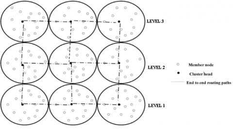
Figure 1. Different cluster head connection with various clusters
Cluster heads hierarchical structure is illustrated in Figure 1. The cluster head at level1 sends the information to the base station via the cluster head at level 2 and level 3. The sensors in level 2 and level 3 region can aggregate the data by their corresponding cluster head which is then forwarded to the base station. Here, minimum hop count is chosen as next higher level for routing. The members involved in all the clusters forward the information to the cluster head within allocated TDMA schedule to avoid collisions. It is also noted that in all the clusters, the cluster head is mostly located at the centre region of the cluster. In a cluster, almost all the nodes can communicate with cluster head within one or two hops. In addition to the location information, node residual energy, number of links connected to the node, distance between the node and the base station. This leads to save the energy of other sensor nodes. Also, the nodes that are not involved in sensing and routing process can make the sensors to sleep mode to save the energy. The role of the cluster head involves three major tasks:
(1) Collect and aggregates the sensed data from the member nodes and remove the redundant values.
(2) Allocate Time Division Multiple Access (TDMA) slot to avoid collisions from individual member sensor node to gather the data.
(3) Forward the aggregated data to the other cluster head or to the base station.
Due to these tasks, energy level of cluster head is decreasing slowly. Hence, cluster head is rotated periodically to reduce the burden of an individual sensor node.
3.2 Multipath routing
The Multipath routing is defined as the routing in which the path is established between the source node and the destination node in several ways. The name ‘Multipath’ implies that the source to destination has many alternative paths. This helps to avail many advantages such as fault tolerant and security of the network.
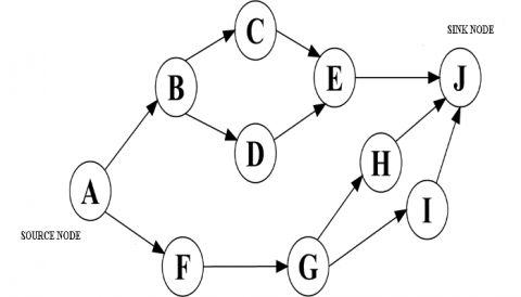
Figure 2. Multipath routing scheme
In Figure 2, nodes ‘A’ and ‘J’ are designated as source and sink nodes respectively. The nodes ‘B’, ‘C’, ‘D’, ‘E’, ‘F’, ‘G’, ‘H’ and ‘I’ are considered as the intermediate nodes.
The possible routing schemes are,
A-B-C-E-J
A-B-D-E-J
A-F-G-H-J
A-F-G-I-J
The above all routing pairs reach the destination with a maximum of four hops. Based on the routing protocols used, the routing path can be chosen. If any of the path is broken, the data transmission process is still continuous via the other possible routing paths. Multipath routing helps to route the data efficiently to the destination through many paths. In case of single routing path, due to the failure (link broken) between intermediate nodes, the data cannot be reached the destination. This affects the packet delivery ratio of the network. This can be avoided by multipath routing.
3.3 Neighbour node selection phase
It is very important to route the messages efficiently to the destination node from the member sensor node. The neighbour node selection phase involves a major role in this proposed protocol. Neighbour node sensors in a cluster are not always awake due to the limited energy level of the sensors. During this phase, the sensor nodes can identify the neighbour node for routing the information. This neighbour node data is updated on the routing table. This indicates that the number of links connected to the certain node. Each member sensor node has its own routing table information to update the information about the destination node, energy level and also the node weight. The main purpose of the proper neighbour node selection is to route the data efficiently. Neighbour node with good link quality is another important factor in WSN. In case, the neighbour node is selected with bad link quality leads to energy wastage and packet loss. Due to this bad link quality, reliability of the network is decreased. Hence, it is important to select the neighbour node with good link quality.
Neighbour node can be found by broadcasting neighbour_msg to the other sensors. After the node receives this neighbour_msg, it adds the node as source node and reply with an acknowledgement (ack) packet. After receiving, all the ack packet from the sensors, neighbour table is constructed and thus, neighbour node is found. Each cluster head broadcasts advertisement (adv) packet to the cluster members to join with the cluster head. Cluster head calculates the distance between the cluster member sensor and itself. If the distance between them exceeds the threshold value, multi-hop routing is used to reach the cluster head from the sensors. Within two hops, the sensor node reaches the cluster head. The node which may not reach within two hops to the cluster head is not considered for sensing. If this is considered, the node consumes more energy due to more number of hops involved to reach the cluster head.
3.4 Fault tolerability
Generally, all the sensor nodes in the network are energy dependent. So, it is very much important to use the energy effectively. As part of energy saving scheme, proper routing also plays a major role in WSN. Data forwarding through various sensors can consume some amount of energy. Through the neighbour node sensors, path is established from the sensing event region to the final destination node/ base station. In the proposed scheme, due to central location of cluster head node, almost all the sensors reach the cluster head with maximum two or three hops. Due to failure of the forwarder intermediate node, the data send by the source node may not reach the cluster head. So, the source node can form the multipath routing to the cluster head node. In case of path failure, another path is established with other neighbour nodes between the source sensor nodes to the cluster head. During path failure, the source node finds an alternate routing based on the RERR msg received from the previous forwarder node. After received this message, the value of neighbour nodes energy can be obtained from the routing table.
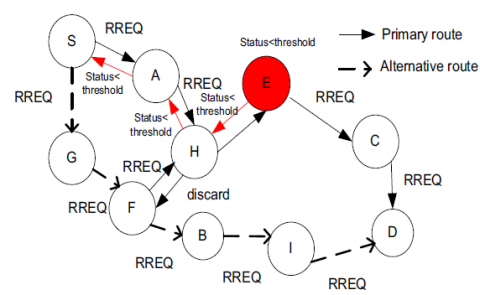
Source node easily establishes another routing path from the source node to the central location of the cluster head. In few cases, it is assumed that the cluster head is located at the corner of the cluster region. In these situations, sensors may take more number of hops to attain the cluster head. Prior finding of an alternate path from source to the cluster head node helps to decrease the route recovery time. In order to distribute the workload, cluster head selection is periodically changed. This causes the changes of path selection with neighbour node and the source sensor node. The proposed scheme is suitable for these cluster head positions. This is illustrated in Figure 3.
Rreq-Route Request
Rrep- Route Reply
Figure 3. Multipath fault tolerant routing scheme
In this work, the first order radio model is used to model the energy dissipation. When the distance between the transmitter and receiver is less than a threshold value ‘d0’, the free space model (d2 power loss) is employed. Otherwise the multipath fading channel model (d4 power loss) is used. Equation (1) shows the amount of energy consumed for transmitting ‘l’ bits of data to the distance‘d’, while (2) represents the amount of energy consumed for receiving ‘l’ bits of data.
$\mathrm{E}_{\mathrm{Tx}}(\mathrm{l}, \mathrm{d})=\left\{\begin{array}{l}1^{*} \mathrm{E}_{\mathrm{elec}}+1^{*} \varepsilon_{\mathrm{fs}} * \mathrm{d}^{2}, \mathrm{d}<\mathrm{d}_{0} \\ 1^{*} \mathrm{E}_{\mathrm{elec}}+1^{*} \varepsilon_{\mathrm{mp}}^{*} \mathrm{d}^{4}, \mathrm{d} \geq \mathrm{d}_{0}\end{array}\right.$ (1)
$\mathrm{E}_{\mathrm{Rx}}(\mathrm{l}, \mathrm{d})=\mathrm{l}^{*} \mathrm{E}_{\text {elec }}$ (2)
The threshold value d0 could be obtained via (3).
$\mathrm{d}_{0}=\sqrt{\frac{\varepsilon_{\mathrm{fs}}}{\varepsilon_{\mathrm{mp}}}}$ (3)
where,
$E_{\text {elec }}$ -Energy consumption per bit in the transmitter and receiver circuits.
$\varepsilon_{\mathrm{fs}}-$ Energy consumption factor for free space.
$\varepsilon_{\mathrm{mp}}$ -Energy consumption factor for multipath radio models.
The performance of the proposed scheme is simulated in Network Simulator 2 (NS 2). The initial energy given to all the nodes are 2 Joules. First order radio model is employed here. The position of the base station is fixed at the centre of the network area. The simulation parameters are listed in Table 1.
Table 1. Simulation environment
|
Simulation Parameters |
Specifications |
|
Simulation tool used |
Network Simulator 2 (NS 2) |
|
Number of nodes |
100 |
|
Simulation area |
500 m * 500 m |
|
Initial energy |
2 Joules |
|
Energy consumed / received per bit |
50 nJ/ bit |
|
Base station position |
(250, 250)m |
|
Free space energy consumption factor |
10 pJ/ bit/ m2 |
|
Multipath radio model energy consumption factor |
0.0013 pJ/bit/m4 |
5.1 Simulation scenario
The simulation scenario is assumed as follows:
5.2 Network animator (NAM) window
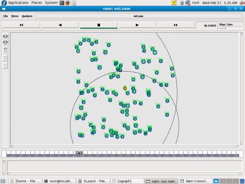
The network animator window depicts the random organization of the sensor nodes in a given area (500m* 500m). Red colour circle indicates the position of the base station which is assumed to be at the centre position.
Figure 4. Network animator (NAM) window
Sensors are randomly deployed. Here, cluster heads are nominated in different levels: level 0, level 1 and level 2. In a cluster, the nodes that are communicated to the cluster head with a maximum of two hop distance. Cluster head is fixed almost at the central location in all the clusters. Cluster head can form the hierarchy for data transmitting from lower level CH to base station through higher level CH. Sensors placed for sensing, routing the data to the corresponding cluster head and then the cluster head collectively sends the information/data/ packets to the base station. Black colour circle indicates the updating of routing table by the sensors as illustrated in Figure 4.
5.3 Number of rounds vs number of alive nodes
Figure 5 indicates that the number of nodes that are alive in the network. From Figure 5, it is clearer that the number of alive nodes slowly moves to dead condition when the number of rounds is increased. Red and Green colour lines show the existing and the proposed scheme of the alive nodes in the network respectively.
Figure 5. Number of rounds vs number of alive nodes
It is clearer that the existing (Red) scheme reached zero at almost after 1310 rounds. Due to no nodes are in alive condition, the entire network cannot be functioned. However, in the proposed (Green) scheme the alive nodes are 38 at 1310 rounds. Hence, the proposed protocol enhances the lifetime of the network with more number of alive nodes when compared with the existing protocol.
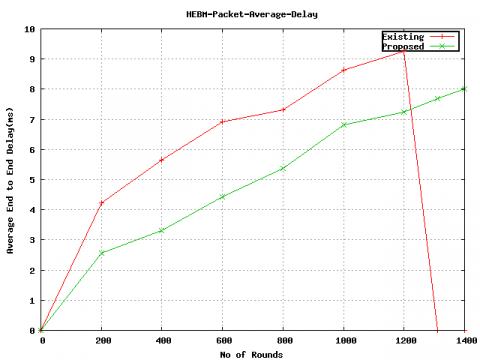
5.4 Number of rounds vs average end-to-end delay
Figure 6. Number of rounds vs average end-to-end delay (ms)
The total time taken by the sensor node from the cluster member node to cluster head and from cluster head to the base station is kept as low. For an efficient network, delay should be as much as low. Red and Green colour lines specify the existing and the proposed schemes of end to end delay in the network respectively. Delay happens due to improper selection of cluster head and also improper routing path selection. In our proposed scheme, cluster heads are nominated based on the following metrics: location information, remaining energy, distance of the node from the cluster head and the distance of cluster head from the base station. These two kinds of distance supports the proper routing path structure from cluster head to base station or to other cluster head results in shorter end to end delay. From Figure 6, it is clearer that the proposed protocol has less end to end delay when compared to the existing protocol. Figure 6 evidently indicates that the proposed scheme outperforms the existing scheme in terms of end-to-end delay.
All the sensor nodes in the network are dead at 1310 rounds in the existing scheme. Hence, no sensor is alive to sense the data for transmission and routing. But in the proposed protocol, 38 nodes are still alive to sense and route the data. So, delay is present in the proposed protocol.
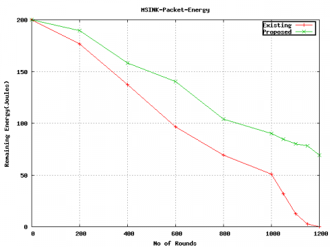
5.5 Number of rounds vs remaining energy
Remaining energy / Residual energy is the energy remain unspent by the sensor nodes in the network. When the number of rounds increases, residual energy decreases. At 1310 rounds, the residual energy of the existing protocol reaches zero. At that instant, the proposed protocol has some amount of energy helps to route the data. Red and Green colour lines specify the existing and the proposed scheme of the network respectively. From Figure 7, it is evident that the proposed protocol outperforms the existing protocol in terms of remaining energy. Initially, the total remaining energy in the network is 200 joules. When the nodes start sensing, the energy level slowly decreases with increase in number of rounds. Not only energy is used for sensing, but also used for routing purpose. This affects entire network lifetime. Hence, energy is the most desirable factor in wireless sensor network. So, the energy level of the sensor is used very much effectively and efficiently. The nodes that are not involved in sensing and routing turn into sleep state.
Figure 7. Number of rounds vs remaining energy
5.6 Number of rounds vs packet delivery ratio
Packet delivery ratio should be as much as high for an efficient network. When the number of rounds increases, packet delivery ratio gradually decreases.
Red and Green colour lines indicate the existing and the proposed scheme of packet delivery ratio of randomly deployed wireless sensor network respectively. At 1310 rounds, all the sensors in the existing scheme is dead. Hence, there is unavailable of sensor for data routing. But in case of proposed technique, due to alive sensors at 1310 rounds, data is routed to the base station via the cluster head. Figure 8 demonstrates that the proposed scheme outperforms the existing scheme in terms of packet delivery ratio in wireless sensor network. The data gathered by the sensor can forward the information to the cluster head and from cluster head to the base station. Maximum amount of sensed data should reach the destination node implies that the packet delivery ratio is high.
Figure 8. Number of rounds vs packet delivery ratio
With the help of location information, remaining energy, weight, distance of a node with neighbour and the distance from base station to a node, cluster head is selected. This cluster head selection balances the energy consumption by equally allocating the workload among sensors. The simulation result illustrates that the proposed protocol has increased the number of alive nodes, lower end to end delay, increase in residual energy and high packet delivery ratio of the wireless sensor network. It is clearer that the number of alive nodes measured in the proposed protocol is 68 where the existing protocol has only 40 nodes are alive at 1000 rounds. When the number of rounds increases, alive nodes gradually lose its energy level and all the nodes are dead at 1310 rounds in case of existing protocol. In the proposed scheme, 38 nodes are still alive at 1310 rounds. This leads to enhance the overall network lifetime in WSN. Due to zero energy level at 1310 rounds in the existing method, the parameters such as alive nodes, delay and data transmission are zero. From the simulation results, it is clearer that the proposed energy efficient clustering scheme and fault tolerant routing achieves better performance in terms of alive nodes, end to end delay, residual energy and packet delivery ratio. Efficient energy saving leads to increase in more number of alive sensor node helps to improve the entire network lifetime.
|
ADPV |
Adaptive Disjoint Path Vector |
|
CH |
Cluster Head |
|
DBI |
Davies-Bouldin Index |
|
ECM |
Evolutionary Clustering Method |
|
HEBFTMR |
Hierarchical Energy Balanced Fault Tolerant Multipath Routing Protocol |
|
NAM |
Network Animator |
|
NS |
Network Simulator |
|
RREP |
Route Reply |
|
RREQ |
Route Request |
|
RSS |
Received Signal Strength |
|
TDMA |
Time Division Multiple Access |
|
WSN |
Wireless Sensor Network |
|
WSNs |
Wireless Sensor Networks |
[1] Sajjanhar, U., Mitra, P. (2007). Distributive energy efficient adaptive clustering protocol for wireless sensor networks. International Conference on Mobile Data Management, IEEE Computer Society, Mannheim, Germany, 326-330. https://doi.org/10.1109/MDM.2007.69
[2] Awad, M., Abuhasan, A. (2016). A smart clustering based approach to dynamic bandwidth allocation in wireless networks. International Journal of Computer Networks & Communications, (8): 73-86.
[3] Gherbi, C., Aliouat, Z., Benmohammed, M. (2016). An adaptive clustering approach to dynamic load balancing and energy efficiency in wireless sensor networks. Energy, (114): 647-662. https://doi.org/10.1016/j.energy.2016.08.012
[4] Hua, C.Q., Yum, T.S.P. (2008). Optimal routing and data aggregation for maximizing lifetime of wireless sensor networks. IEEE ACM Transactions in Networking, (16): 892–903. https://doi.org/10.1109/TNET.2007.901082
[5] Deniz, F., Bagci, H., Korpeoglu, I., Yazıcı, A. (2016). An adaptive energy aware and distributed fault tolerant topology control algorithm for heterogeneous wireless sensor networks. AdHoc Networks, (44): 104-117. https://doi.org/10.1016/j.adhoc.2016.02.018
[6] Xie, D.F., Zhou, Q.W., You, X., Li, B.Q., Yuan, X.B. (2013). A novel energy efficient cluster formation strategy: from the perspective of cluster members. IEEE Communication Letters, (17): 2044-2047. https://doi.org/10.1109/LCOMM.2013.100813.131109
[7] Ozger, M., Alagoz, F., Akan, O.B. (2018). Clustering in multi-channel cognitive radio adhoc and sensor networks. IEEE Communications Magazine, (56): 156-162. https://doi.org/10.1109/MCOM.2018.1700767
[8] Liu, J., Li, J., Niu, X.G., Cui, X.H., Sun, Y.C. (2015). Green OCR: An energy-efficient optimal clustering routing protocol. The Computer Journal, (58): 1344-1359. https://doi.org/10.1093/comjnl/bxu052
[9] Ashrafian, V., Harounabadi, A., Sadeghzadeh, M. (2014). A new method for reducing energy consumption in wireless sensor networks using fuzzy clustering and fault tolerance. International Journal of Computer Applications Technology and Research, (3): 109–113. https://doi.org/10.7753/IJCATR0302.1005
[10] Alan Boyd, W.F. (2010). Node Reliance: An approach to extending the lifetime of wireless sensor networks. Ph.D Thesis, School of Computer Science, University of St. Andrews, Scotland.
[11] Azharuddin, M., Kuila, P., Jana, P.K. (2015). Energy efficient fault tolerant clustering and routing algorithms for wireless sensor networks. Computers & Electrical Engineering, (41): 177-190. https://doi.org/10.1016/j.compeleceng.2014.07.019
[12] Kumaran, S.R., Nagarajan, G., (2017). Energy efficient clustering approach for heavy data traffic in wireless sensor networks. AMSE Journals, Series: Advances D, 22(1): 98-112.
[13] Zhang, K.S., Zhong, L., Tian, L., Zhang, X.Y., Li, L. (2017). DBIECM-an Evolving Clustering Method for Streaming Data Clustering. Advances B (Signal Processing and Pattern Recognition), AMSE Journals, 60(1): 239-254. https://doi.org/10.18280/ama_b.600115
[14] Sivakumar, S., Venkatesan, R. (2014). Cuckoo Search with Mobile Anchor Positioning (CS-MAP) algorithm for error minimization in wireless sensor networks. AMSE Journals, Series Advances D, 19(1): 33-51.
[15] Kumaran, S.R., Nagarajan, G. (2017). Enhancement of network lifetime in wireless sensor networks using Energy Efficient Mobile Sink Based Routing Protocol (EEMSBRP). International Journal of Wireless Communication, (9): 45-49.
[16] Azharuddin, M., Kuila, P., Jana, (2015). Energy efficient fault tolerant clustering and routing algorithms for wireless sensor networks. Computers & Electrical Engineering, (41): 177-190. https://doi.org/10.1016/j.compeleceng.2014.07.019
[17] Kumaran, S.R., Nagarajan, G. (2013). Enhancement of network lifetime in Wireless Sensor Networks (WSNs) using Residual energy. International Journal of Image mining, (2): 116-128.
[18] Faheem, M., Asri, B., Ali, S., Shahid, M., Sakar, L. (2013). Energy based efficiency evaluation of cluster-based routing protocols for Wireless Sensor Networks (WSNs). International Journal of Software Engineering and Its Applications, (7): 249-264.
[19] Gong, D., Yang, Y., Pan, Z. (2013). Energy-efficient clustering in lossy wireless sensor networks. Journal of Parallel and Distributed Computing, (73): 1323–1336. https://doi.org/10.1016/j.jpdc.2013.02.012
[20] Sebastian, M.P. (2007). Protocol architecture for end-to-end security between server and wireless client. AMSE Journals, Advances D , 23(3): 82-97.
[21] Bhattacharjee, S., Bandyopadhyay, S. (2013). Lifetime maximizing dynamic energy efficient routing protocol for multihop wireless networks. Simulation Modelling Practice and Theory, (32): 15–29. https://doi.org/10.1016/j.simpat.2012.11.006
[22] Soleimani, M., Ghasemzadeh, M., Sarram, M.A. (2011). A new cluster based routing protocol for prolonging network lifetime in wireless sensor networks. Middle-East Journal of Scientific Research, (7): 884–890.