Badia Ghernaout | Said Bouabdallah* | Aissa Atia | Müslüm Arıcı
OPEN ACCESS
Flow convection in agriculture greenhouse is one of the most important factors on the growth and fruiting of plants. The present work focused on natural convection in an open greenhouse heated by ridge tubes in presence of plants. Analyses are performed for different boundary conditions imposed at the roof such as constant temperature, convective heat flux, and convective and radiative heat flux. The governing equations comprising continuity, momentum and energy equations are solved by Ansys-Fluent software. In each case, the average velocity and temperature of the air are determined. The obtained results are presented in terms velocity and temperature profiles. Isothermal lines and velocity vectors showed that by increasing the convective heat transfer coefficient, the average temperature and average airflow velocity decrease. The outcomes of this study help build greenhouses with dimensions and materials to suitable for the given external conditions.
airflow, convection, 3D simulation, flow trajectories, heat transfer
Since the world’s population is constantly increasing, production capacity requires achieving sufficiency. To increase productivity and increase yields, sustainable agriculture has become one of the leading ideas for global ambitions. Sustainable agriculture rests on three important points: energy, cost, and environmental impact. Greenhouses are used to increase agricultural production and are among the most energy-consuming sectors on the one hand. On the other hand, they are among the most profitable sectors.
Greenhouse crops are 10 to 20 times better than external gardening [1]. The cost of sustainable agriculture is high because it includes the cost of labor, fertilizers, and energy inputs for heating and lighting. The largest amount of solar radiation is collected inside the greenhouse when it heads east and west; especially in winter [2, 3]. The use of dual thermal screen or double glazing allows us to improve energy saving in greenhouses and the rate of energy reduction is about 60%. When using a fully enclosed greenhouse without ventilation, the rate of energy drop reaches about 80% [4].
There are many experimental and numerical studies carried out in this field. Tiwari and Dhiman [5] developed a mathematical model for winter greenhouse, which was useful especially for greenhouses in cold areas in winter. Greenhouse cultivation enables to succeed in agricultural crops because solar radiation is sufficient throughout the year. Arithmetic results showed that it is sufficient in winter nights to supply two southern and northern glass walls and a glass roof that enables us to provide sufficient energy, reduces heat loss and increases the air inside the greenhouse.
Van Beveren et al. [6] proposed a novel dynamic model of heating and cooling systems to minimize the energy need of a rose greenhouse. The researchers concluded that having less natural ventilation and more heating on cold days and more natural ventilation and less heating on warm days can reduce energy consumption. They stressed out that energy inputs in greenhouse gases decrease by lowering temperature and humidity as well. Seginer et al. [7] developed a typical greenhouse without production by adding 6 elements to the double cover, and also developed highly absorbent panels. They concluded that the double cover maintains the greenhouse temperature more effectively than a single cover. They also found that higher absorption plates increase the heat flow compared to the normal. Ghernaout et al. [8] conducted a numerical study of natural convection in a closed greenhouse model heated by pipes. They calculated each of the following parameters in the greenhouse: thermal and dynamic flow, average temperature and average speed. The researchers concluded that the obtained results relate to the experimental data. These results also help farmers to create greenhouses with dimensions and materials to suit all external. Boulard et al. [9] studied the mono Chappelle greenhouse, concerned themselves with the distribution of flow and temperature that stimulates ventilation with one or two holes on the greenhouse surface. The results revealed that the airflow is characterized by one loading ring for one or two holes on the surface with floor heating and high velocity in the ceiling and floor. It was concluded that temperature gradients cause air regeneration, which is the origin of the convection movement. Besides, they reported that the mean components of the air velocity and temperature and the shape of the convective loop were compatible with the experimental results. Then, Boulard et al. [10] built a greenhouse model with reduced scale to study airflow and temperature characteristics in the greenhouse which is heated from floor. They showed that, a main flow circulation was formed in the greenhouse and the air in the centre was still. Bartzanas et al. [11] studied the tunnel greenhouse, and they were concerned with the effects of temperature patterns inside the greenhouse, as well as how the screen affects air flow and climatic conditions inside the greenhouse. They concluded that the screen a remarkable influence on the greenhouse climate, reducing the air velocity and airflow rate by 50% which leads to considerable temperature rise. The wind direction had a more profound effect on the airflow and temperature distribution particularly for the greenhouse having an insect screen.
Chen and Cheng [12] conducted experimental and numerical investigations of the behaviour of heat transfer and buoyancy flow within an oblique arc-shaped container considering different inclination angles and Grashof numbers. They also built an experimental setup that uses flow visualization technology, and to monitor the flow pattern. Later, Impron et al. [13] built six models of greenhouses in the tropical lowlands. The study indicated that the vapour water pressure and air temperature were satisfactorily consistent. They concluded that such models could be employed as a design tool for tropical lowland greenhouses.
Using a commercial CFD code, Tong et al. [14] studied temperature variation within a solar greenhouse regarding external climatic conditions such as solar insolation and outdoor, soil and sky temperatures. It was reported that a reasonable temperature in the greenhouse could be attained even when the outdoor temperature dropped below zero. Attar and Farhat [15] developed a thermal model to study the efficiency of the solar water system utilized for heating a greenhouse in Tunisia. It was found that the key factors are heat exchanger length and flow rate.
Recently, Bouabdallah etal. [16] conducted a numerical study of natural convection using the commercial CFD package in a closed greenhouse model heated by tubes. They calculated each of the following parameters in the greenhouse: thermal and dynamic flow, average temperature and average velocity. The researchers concluded that the obtained results relate to the experimental data. These results also help farmers to create greenhouses with dimensions and materials to suit all external conditions.
After a comprehensive bibliographic study, it has been noticed that there are a few numerical studies related to the natural convection in the greenhouses in the presence of plants, that is motivation of this work, as an extension of our previous work of Bouabdallah et al. [16]. For that, this study aims to investigate air flow and temperature characteristics in an open greenhouse, using Ansys-Fluent software. A particular attention has been devoted to the natural convection inside open greenhouse with plant cover, where different boundary conditions imposed on the roof are considered. The rest of the paper is structured as follows: first the description of physical problem and mathematical formulation are presented, following by presenting the simulation results and interpretations. Finally, the conclusion and perspectives are given in the last section.
The geometry of the greenhouse considered in the study is represented in Figure 1. The height, width and depth of greenhouse is respectively H1 = 2 m, W = 2.2 m and D = 1.5 m. In these conditions, the medium is completely transparent. Also, we have considered the air in the greenhouse to be an ideal gas with a temperature value equal to T = 300 K and a pressure value equal to P = 1 atm.
The greenhouse is heated by circulating hot waters through four tubes with diameter of 32 mm which are placed near the floor with a height of h = 60 mm. A heat flux of q = 200 W/m² is considered for each tube. The plant cover consists of a row of tomato plants located in the center of the greenhouse between the heating tubes with a height of 1.3 m and a width of 0.58 m. The buoyancy force causes the heat flow from the contents of the heating tubes and the absorption of solar energy onto the ground. Greenhouse walls are made of glass as semi-transparent material.
Figure 1. Geometry of the model
It was assumed that the heat transfer from lateral, front and rear walls, and ground is not taken into account, i.e. these walls are taken adiabatic. The velocities (u, v, w) on the walls are also equal to zero for the model configurations. The analysis was performed for various boundary conditions imposed on the roof. In the first case (BC 1), a constant temperature (T = 300 K) is considered. In the second case (BC 2), the boundary condition is the convective heat transfer, which is given by:
$\mathrm{q}=\mathrm{h}\left(\mathrm{T}-\mathrm{T}_{0}\right)$ (1)
where, h is the heat transfer coefficient (h = 5 W/m².K) and T0 is the outdoor temperature (300 K). The third case (BC 3) and fourth case (BC 4) are the same as BC 2 with a distinction in the magnitude of convective boundary condition, which is h = 10 W/m².K and 20 W/m².K, respectively. The last case (BC 5) is a mixed boundary condition including both convective and radiative heat transfer as follows:
$\mathrm{q}=\mathrm{h}\left(\mathrm{T}-\mathrm{T}_{0}\right)+\varepsilon \sigma\left(\mathrm{T}^{4}-\mathrm{T}_{0}^{4}\right)$ (2)
where, ε is the external emissivity (0.9) and σ is the Stefan-Boltzmann constant (5.672´10-8 W/m².K4). In this case, the convective heat transfer coefficient and outdoor temperature are taken the same as in Case 2 (i.e. h = 5 W/m².K and T0 = 300 K). To simulate the airflow under the greenhouse, we have used the software Ansys-Fluent, which solves the Navier-Stokes equations ([16, 17]) using finite volume method. It is proposed to assimilate the plant cover to a porous medium. In addition, the software accounts a standard way the porous medium with the discretization of the Darcy and Forshheimer equations. The permeability intrinsic of the porous medium K = 0.884 m2 and the coefficient of non-linear pressure drop CF = 1 are used. These parameters are determined experimentally on tomato plants by Haxaire [18]. The physical phenomena are described by the conservation equations represented by the general transport equation:
$\frac{\partial(u \varphi)}{\partial x}+\frac{\partial(v \varphi)}{\partial y}+\frac{\partial(w \varphi)}{\partial z}=\Gamma. \nabla^{2} \varphi+S_{\varphi}$ (3)
where, φ denotes a typical physical parameter in flow field, the expression of which can be found in Ould Khaoua et al. [19]. u, v and w represent the velocity vector components, Γ stands for the diffusion coefficient, and Sφ denotes the source term. The velocity vector V and temperature T are obtained by solving mass, momentum, and energy conservation equations. The three-dimensional flow is assumed to be steady, and incompressible. The thermophysical properties of the air are assumed constant, except for density, which varies with temperature where the Boussinesq assumption is valid.
Before starting the numerical simulation, we have studied the effect of mesh density. For this, we have tested five meshes with different sizes defined by 303, 403, 503, 603, and 703 nodes for greenhouse without tubes. Figure 2 presents the profile of the temperature in the middle of the greenhouse. From the results, it can be observed that the average temperature at the three last cases present stable results. This fact allows us to choose any one of them. Thus, the smaller mesh 50×50×50 has been chosen since it requires less computational resources to obtain the solution.
Figure 2. Comparison of temperature profiles for different sizes of meshes
A validation study is conducted by considering the same conditions given in the study of Roy et al. [20]. Figure 3 compares the velocity vectors obtained by our numerical model with those acquired experimentally. The figure indicates that the obtained results present approximately the same behaviour as the experimental results, thus confirms the credibility of the numerical model for the analysis.
Figure 3. Comparison of velocity vector fields obtained in the present numerical model (top) with the experimental results (down) of Roy et al. [20]
5.1 A greenhouse with ridge
Figure 4 shows the velocity vector fields inside the greenhouse moving in the direction of the watch in the presence of the small vortexes on the right side of the greenhouse for the case of ridge 50%. From these results, a low velocity has been observed in the middle, lower right and left. In the case of 100% ridge, a large vortex causes the particles to circulate in the center of the greenhouse in the direction of the watch. The velocity is almost zero in the middle and the lower part right and left. However, it increases near the roof side.
The velocity profile according to the Y-axis for a ridge of 50 and 100% with imposed roof temperature is presented in Figure 5. From these results and due to the opening orientation, a great variation in the velocity on the right side of the greenhouse appears. On the right side of the roof and due to the airflow, the velocity is more significant for the opening of 100%, compared to 50%.
Figure 4. Velocity vector fields in the greenhouse for imposed roof temperature (z = 1.75 m), for 50% ridge (a) for 100 % ridge
Figure 5. Velocity profiles according to Y-axis for a ridge of 50 and 100% with imposed roof temperature (Case 1)
5.2 A closed greenhouse with the presence of a plant
Figure 6 shows the parallel planes of the isothermal lines along the Y axis denoted by Y = 0.06, 0.5, 1, and 1.5 m. From these results, a slight variation in the sides of the closed greenhouse has been observed where the imposed outdoor temperature is 300 K. Near the tubes, the temperature reaches 305 K and a large gradient of temperatures has been noted. For the cases where the greenhouse is subjected to a constant convective flow values equal to h = 5, 10, and 20 W/m².K, a large change in temperature near the tubes is noticed.
a) BC 1: Specified temperature (T = 300 K)
b) BC 2: Convective boundary condition with h = 5 W/m².K
c) BC 3: Convective boundary condition with h = 10 W/m².K
d) BC 4: Convective boundary condition with h = 20 W/m².K
e) BC 5: Mixed boundary condition
Figure 6. Isothermal surfaces in different levels in the greenhouse for various boundary conditions imposed on the roof
a) BC 1: Specified temperature (T = 300 K)
b) BC 2: Convective boundary condition with h = 5 W/m2.K
c) BC 3: Convective boundary condition with h =10 W/m2.K
d) BC 4: Convective boundary condition with h = 20 W/m2.K
e) BC 5: Mixed boundary condition
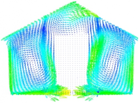
Figure 7. Pathline of particles for different boundary conditions imposed on the roof
a) BC 1: Specified temperature, (Vavg = 13.1 cm/s)
b) BC 2: Convective boundary condition with h = 5 W/m2.K, (Vavg = 13.5 cm/s)
c) BC 3: Convective boundary condition with h = 10 W/m2.K, (Vavg =13.7 cm/s)
d) BC 4: Convective boundary condition with h = 20 W/m2.K, (Vavg = 14.4 cm/s)
e) BC 5: Mixed boundary condition (Vavg = 14.1 cm/s).
Figure 8. Velocity vectors at z = 0.75 m, for different cases of greenhouse
Under the effect of the heat flux emitted, a low temperature gradient appears next to the roof. In these cases, the corresponding average temperatures are respectively equal to 310, 307, and 306 K. In the case of a mixed convection-radiation boundary condition (i.e. BC 5), a large temperature gradient is revealed near the hot tubes and in the center of the greenhouse. Indeed, a small variation next to the roof has been observed and the average temperature is equal to 307 K.
Some trajectories of the particles in the greenhouse are shown in Figure 7 for the mentioned boundary conditions. As seen in the figure, the convection between the tubes and the roof establishes two main vortexes which are rotating in opposite directions in the left and right sides of the greenhouse. For Case 2 (h = 5 W/m².K), the particles are circulated via small vortexes. With increasing convective heat transfer coefficient on the outer surface of roof, the flow intensifies. For the largest heat transfer coefficient, which is h = 20 W/m².K (Case 4), the particles circulate in opposite directions with great turbulence. In the case of a mixed convection-radiation flow (Case 5), a large turbulence in the left part of the greenhouse appears. In these conditions, the particles circulate in vortex flow due the effect of convection between the tubes and the walls.
Figure 8 shows the velocity vector field in the plane defined by Z = 0.75 m for the considered boundary conditions. It can be seen from the results presented in the referred figure that the velocity is high at ground level and roof, low in the sides of walls and zero in the center. For the different cases, the average velocity values are respectively equal to Vavg = 13.5 cm/s, 14.4 cm/s, and 13.7 cm/s. The velocity remains low in the center of greenhouse except at the roof side for the imposed temperature case (BC 1). For the mixed flow boundary condition case (BC 5), the airflow velocity is high near the tubes and the left wall of the greenhouse. At the top near the roof and in the center, the velocity of airflow is lower with an average velocity Vavg = 14.1 cm/s.
Figure 9-a presents temperature profiles in the Y direction for various boundary conditions. From these results, the temperature reaches 307 K near to the hot tube supplying a heat flow of 200 W/m² and remains constant in the medium. While approaching to the roof, it falls considerably to the roof temperature where it is at about 300 K. The average temperature remains constant at 310 K for h = 5 W/m2.K (BC 2) and it reduces with increasing heat transfer coefficient, namely it is equal to 308 and 307 K for h = 10 and 20 W/m2.K, respectively. In the case of a mixed flow (convection and radiation, i.e. BC 5) imposed on the roof, the temperature of the air on the ground is risen. After that, the temperature decreases considerably in the medium and while approaching the roof, it falls with the value of T = 301 K.
Figure 9-b displays the comparison of horizontal velocity along vertical direction in the greenhouse heated by the tubes in presence of plants for the aforementioned five different boundary conditions. It is evidently seen from the curves plotted in the figure; the profiles have the same profile at the beginning. The results display that the velocity is constant (zero) in the region close to the ground. The highest X-velocity value is observed for the imposed temperature case, (BC 1, T = 300 K) whereas the minimum value is recorded for the convective boundary condition with the lowest value of h = 5 W/m2.K (BC 2).
(a)
(b)
Figure 9. Temperature profiles (a) and X- component velocity profiles (b) along Y-axis (X =1.1 m) for different boundary conditions
In this work, natural convection in a greenhouse is studied to analyze the airflow and temperature patterns in a greenhouse. The simulations are performed for several configurations of thermal conditions imposed on the roof including constant temperature, convective boundary conditions with different convective heat transfer coefficients, and mixed (radioactive and convective) boundary conditions in the presence of plants in the greenhouse. The main results are given below:
In the future work, we can study the ventilation velocity and doing the experiment on prototype greenhouse.
The authors gratefully acknowledge the Directorate General of Scientific Research and Technological Development (DGSRTD) – to support this work, and fund the LME laboratory for carrying out research.
|
CP |
specific heat at constant pressure, J. kg-1. K-1 |
|
|
D |
depth of the greenhouse, m |
|
|
g |
gravity acceleration, m. s-2 |
|
|
h |
convective heat transfer coefficient, W.m-2. K-1 |
|
|
H |
height of the greenhouse, m |
|
|
k |
thermal conductivity, W.m-1. K-1 |
|
|
q |
convective heat flux, W. m-2 |
|
|
W |
width of the greenhouse, m |
|
|
Greek letters |
||
|
ε |
external emissivity |
|
|
b |
volumetric expansion coefficient, K-1 |
|
|
υ |
kinematic viscosity, m-2. s |
|
|
σ |
Stefan-Boltzmann constant, W.m-2. K-4 |
|
[1] Vadiee, A., Martin, V. (2012). Energy management in horticultural applications through the closed greenhouse concept, state of the art. Renewable and Sustainable Energy Reviews, 16(7): 5087-100. https://doi.org/10.1016/j.rser.2012.04.022
[2] Rosa, R., Silva, AM., Miguel, A. (1989). Solar irradiation inside a single span greenhouse. Journal of Agricultural Engineering Research, 43: 221-229. https://doi.org/10.1016/S0021-8634(89)80020-4
[3] Abdel-Ghany, A.M. (2011). Solar energy conversions in the greenhouses. Sustainable Cities and Society, 1(4): 219-226. http://dx.doi.org/10.1016/j.scs.2011.08.002
[4] Vadiee, A, Martin, V. (2014). Energy management strategies for commercial green- houses. Applied Energy, 114: 880-888. https://doi.org/10.1016/j.apenergy.2013.08.089
[5] Tiwari, G.N., Dhiman, N.K. (1986). Design and optimization of a winter greenhouse for Leh-type. Energy Conversion and Management, 26(1): 71-78. https://doi.org/10.1016/0196-8904(86)90034-8
[6] Van Beveren, P.J.M., Bontsema, J, Van Straten, G., Van Henten, E.J. (2015). Minimal heating and cooling in a modern rose greenhouse. Applied Energy, 137: 97-109. https://doi.org/10.1016/j.apenergy.2014.09.083
[7] Seginer, I., Dvora, K., Peiper, U.M., Levav, N. (1988). Transfer coefficients of several polyethylene greenhouse covers. Journal of Agricultural Engineering Research, 39(1): 19-37. https://doi.org/10.1016/0021-8634(88)90163-1
[8] Ghernaout, B., Attia, MEH., Bouabdallah, S., Driss, Z., Benali, M.L. (2020). Heat and fluid flow in an agricultural greenhouse. International Journal of Heat and Technology, 38(1): 92-98. https://doi.org/10.18280/ijht.380110
[9] Boulard, T., Haxaire, R., Lamrani, M.A., Roy J.C., Jaffrin, A. (1999). Characterization and modelling of the air fluxes induced by natural ventilation in a greenhouse. Journal of Agricultural Engineering Research, 74(2): 135-144. https://doi.org/10.1006/jaer.1999.0442
[10] Boulard, T., Wang, S., Haxaire, R. (2000). Mean and turbulent air flows and microclimatic patterns in an empty greenhouse tunnel. Agricultural and Forest Meteorology, 100(2-3): 169-181. https://doi.org/10.1016/S0168-1923(99)00136-7
[11] Bartzanas, T., Boulard, T., Kittas, C. (2002). Numerical simulation of the airflow and temperature distribution in a tunnel greenhouse equipped with insect-proof screen in the openings. Computers and Electronics in Agriculture, 34(1-3): 207-221. https://doi.org/10.1016/S0168-1699(01)00188-0
[12] Chen, C.L., Cheng, C.H. (2002). Buoyancy-induced flow and convective heat transfer in an inclined arc-shape enclosure. International Journal of Heat and Fluid Flow, 23: 823-830. https://doi.org/10.1016/S0142-727X(02)00189-3
[13] Impron, I., Hemming, S., Bot, G.P.A. (2007). Simple greenhouse climate model as a design tool for greenhouses in tropical lowland. Biosystems Engineering, 98(1): 79-89. https://doi.org/10.1016/j.biosystemseng.2007.03.028
[14] Tong, G., Christophe, D.M., Li, B. (2009). Numerical modelling of temperature variations in a Chinese solar greenhouse. Computers and Electronics in Agriculture, 68(1): 129-139, https://doi.org/10.1016/j.compag.2009.05.004
[15] Attar, I., Farhat, A. (2015). Efficiency evaluation of a solar water heating system applied to the greenhouse climate. Solar Energy, 119: 212-224. https://doi.org/10.1016/j.solener.2015.06.040
[16] Bouabdallah, S., Chati, D., Ghernaout, B., Atia, A., Laouirate, A. (2016). Turbulent mixed convection in enclosure containing a circular/square heat source. International Journal of Heat and Technology, 34(3): 446-454. https://doi.org/10.18280/ijht.340314
[17] Bouabdallah, S., Ghernaout, B., Bellaouar, A., Bouras, A., Ghazel, A. (2020). 3D forced convection in a box containg two cylindrical heat sources. Advances in Modelling and Analysis B, 63(1-4): 20-25. https://doi.org/10.18280/ama_b.631-404
[18] Haxaire, R. (1999). Caractérisation et modélisation des écoulements d’air dans une Serre, Thèse de Doctorat Nice, France.
[19] Ould Khaoua, S.A., Bournet, P.E., Migeon, C. (2006). Analysis of greenhouse ventilation efficiency based on computational fluid dynamics. Biosystems Engineering, 95(1): 83-98. http://dx.doi.org/10.1016/j.biosystemseng.2006.05.004
[20] Roy, J.C., Bailly, Y., Boulard, T., Haxaire, R. (2000). Experimental study on natural convection in a heated greenhouse. Congrès de la Société Française de Thermique. Lyon, France, Elsevier, Paris–Amsterdam, 11-17.