B. Samuyelu* | P. Rajesh Kumar
OPEN ACCESS
In modern decades, a major problem like echo in recent communication network can be solved by AEC. Even though AEC can be measured as a characteristic significance of identifying system, that is recognizing the path of echo; current teleconferencing and automatic telephones systems enforce numerous restrictions on traditional AFs. The initial limitation occurs when the signals given at input are the signals of speech that are frequently highly colored more willingly when distinguished with white noise; moreover, subsequent one is the impulse response in which the path of echo is sparse and extensive. It further designates that many coefficients are either zero or equivalent to zero. This paper implements a D-MVS-SNSAF technique for identifying the echo cancellation systems by adopting NSAF technique. Here, the amount of transitions in the input/output signals was measured for deriving the polynomial order from two sets of audio signals as input. Further, the proposed method is distinguished with conventional algorithms like NSAF, SS-NSAF, VS-NSAF, VS-SNSAF and MVS-SNSAF and enhancement in the implemented method is proved.
AEC, NSAF, weight initialization, subband, D-MVS-SNSAF, stability
AEC is considered as a well-known technique to govern the echoes produced owing to the automatic audio signals [1-3]. According to this method, the AF is employed to recognize the path of echo among the microphone and loudspeaker of the terminal, and subsequently, the output of filter forms an model of the echo that is reduced from the microphone terminal for avoiding the acoustic echo [4-5]. Even if AEC can be assumed as a major application for recognizing systems, teleconferencing systems, and modern hands-free telephones causes numerous limitations on the traditional AFs [6-8].
The initial limitation relies at the input, where the signals of speech that are well colored when compared with white noise; next is the echo path whose impulse response is sparse and long. This denotes that many of the coefficients are either zero or equal to zero [9, 10]. Hence, the familiar method of NLMS is not appropriate for AEC, owing to its rate of convergence for SEP [5]. The best way to simulate convergence is by SAF technique depending on a significant structure of sampling similar to SAFs [11-13]. Further, NSAF is presented that revealed better performance, along with its complexity which is nearer to that of the NLMS algorithm [14-16].
Moreover, a brilliant way to hurry up convergence is to adopt SAF, since it will be able to convert the colored input in to white signals during filter bank study [17-19]. The NSAF technique includes improved convergence when distinguished with NLMS for the colored signals given at input [20-22]. Also, the NSAF’s complication is equivalent when compared with NLMS for a long AF function [23-25]. Subsequently, to achieve both low steady-state error and fast convergence rate, numerous VSS-NSAF techniques were suggested [26]. In recent times, for developing the rate of convergence of NSAF for SEP, the proportionate family was proposed by directly widening the conventional balanced information to the NSAF [27-28].
The major concept of NSAF is to exploit the signals of subbands, produced by its equivalent variances at input subband, for modifying the weights of a full-band AF. It further tends to the NSAF’s decorrelating nature [29]. Anyhow, as the actual NSAF exploits a fixed step-size, it has to execute a trade-off among low mis-adjustment and fast convergence rate. For finding a solution to this issue, an enhanced version of the NSAF, said to be the SM-NSAF [26], has been generated recently [30]. However, the limitations existed in the filtering techniques tends to diminish the performance enhancement of echo cancellation systems.
This paper contributes a technique for solving the problems in echo cancellation systems by deploying an enhanced NSAF technique known as D-MVS-SNSAF method. Here, the number of transitions in the input/output signals is measured for deriving the polynomial order by providing two audio signals as input. The implementation is done by determining the error bound and memorizing error. Subsequent to the execution, the implemented D-MVS-SNSAF technique is distinguished with the traditional methods like NSAF, VS-NSAF, VS-SNSAF, SS-NSAF and MVS-SNSAF techniques. The paper is contributed as follows. Section 2 discusses the related works and reviews done on this topic. Section 3 explains the echo cancellation system and section 4 describes the modeling process of NSAF. Section 5 demonstrates the proposed deterministic initialization. Section 6 illustrates the results and discussions, and section 7 concludes the paper.
versions by inserting the predicted sparseness into the PNSAF and MPNSAF techniques that could suit to the changes of impulse responses in sparseness. Further, depending on the energy argument, a unified equation to assume the SSMS performance of any PNSAF algorithm is enhanced by simulations. Investigational results in AEC have revealed that the implemented algorithms not only displays rapid rate of convergence but also were robust to the change in the impulse response sparseness.
In 2017, Zheng et al. [2] established a relation of RSM-NSAF algorithms in this paper. By exploiting a novel error bound with RSM, this technique obtains an enhanced toughness in opposition to decreased impulsive noises and misalignment in steady-state comparative to predictable SM-NSAF algorithm. Execution in AEC function substantiates the developments of the implemented techniques.
In 2010, Ni et al. [3] suggested an adaptive grouping system to deal with this trade-off. The grouping is done in subband area, and the integration factor that governs the grouping was modified using a stochastic gradient algorithm that made use of the computation of squared subband errors as the computational function. Investigational results illustrated that the grouping method could acquire both small SS-MSE and fast rate of convergence.
In 2016, Yu et al. [4] presented a new SAF technique by reducing cost-utility of Huber which was vigorous. Accordingly, this technique facilitates the method of NSAF, when it performs resembling the method of SSAF merely owing to the occurrence of impulsive noises. Investigational results, by means of dissimilar input signals that are colored in both impulsive noise and free-impulsive surroundings, demonstrates that the implemented method performs more improved than several conventional techniques.
In 2016, Yu et al. [5] proposed a model for acquiring low steady-state error and rapid rate of convergence in AEC, a convex arrangement method of the enhanced balanced NSAF algorithm is implemented. Rather than the gradient technique in the predictable combination hypothesis, the integration factor was made to order by employing the normalized gradient technique that made it further robust to the deviations of signals in subband error.
In 2016, Petraglia et al. [6] introduced a concentrated complexity subband adaptive algorithm that can be adopted to make use of subbandAPA cost function and a sparse subband filter. A variable step-size technique was introduced, thus offering a rapid rate of convergence, at the same time making certain about the small steady-state mis-adjustments.
In 2010, Ni and Li [7] established a VSSM-NSAF from an additional point of observation that was by recuperating the influence of the subband noises from the signals of error in subband of AF to enhance presentation of the NSAF algorithm. The investigational result reveals better computation of the novel technique when distinguished with other various members of the NSAF family.
Table 1. Review on state-of-the-art methods on Echo cancellation techniques with advanced filtering approaches
|
Author [citation] |
Adopted methodology |
Features |
Challenges |
|
Yu and Zhao [1] |
PNSAF |
|
|
|
Zheng et al. [2] |
RSM-NSAF |
|
|
|
Ni et al. [3] |
CNSAF |
|
|
|
Yu et al. [4] |
RVSS-NSAF |
|
|
|
Yu et al. [5] |
CIPNSAF |
|
|
|
Petraglia et al. [6] |
APSAF
|
|
|
|
Ni and Li [7] |
VSSM-NSAF |
|
|
2.2 Review
Table 1 shows the methods, features, and challenges of conventional filtering techniques based on AEC. At first, PNSAF is introduced in [1], where faster convergence rate is obtained, and it is also more robust to the variation in the sparseness of impulse responses. Anyhow, there is only a lower rate of convergence. Moreover, RSM-NSAF has been implemented by Zheng et al. [2], which minimizes the differentiable cost function and enhances the allocation of testing resources. Further, it gains lower steady-state misalignment. However, a slight variation exists among the hypothetical and execution results and also it exhibits slower speed of convergence. In addition, CNSAF algorithm is introduced by Ni and Li [3] that offers quick rate of convergence and attains small SS-MSE, but it needs a trade-off among fast, small SS-MSE and convergence rate. RVSS-NSAF is implemented by Yu et al. [4] that offers quicker convergence rate and reduced SSE and is robust to impulsive noises. However, there is an increased computational complexity and large computational burden in this technique. In addition, CIPNSAF is adopted by Yu and Zhao [5] that offer even transition from the fast filter to the precise filter and further owing to its robustness adaptation of the mixing parameter is achieved. Only a cyclic way overcame the stagnation problem of the CIPNSAF. Moreover, APSAF algorithm is suggested by Petraglia et al. [6] that provides rapid rate of convergence and assures small SS-MSE mis-adjustment together with minimized complications, yet only the non-zero coefficients of the sub-filters are employed. Also, there is no gain by techniques created for sparse impulse responses. Finally, VSSM-NSAF is employed by Ni and Li [7] that provide better steady-state mean-square behavior along with rapid rate of convergence and reduced mis-adjustments, however a positive number should be summed to avoid division by zero. These limitations are considered for enhancing the echo cancellation algorithm effectively for further implementations.
3.1 General model
A linear echo cancellation [31] is due to the coupling among microphone and loudspeaker that are designed by an FIR. AEC targets to evaluate this coupling. The AEC path $\hat{f}(n)$ is further involved with the signal of loudspeaker $x(n)$ for achieving the echo signal as given in Eq. $(1),$ where coefficients of the AF are indicated by $\hat{f}(n)=$ $\left[\hat{f}_{0}(n) \hat{f}_{1}(n) \cdots \hat{f}_{L-1}(n)\right]^{T}, \hat{r}$ is the echo canceled signal and the vector of samples of loudspeaker is indicated by $X(n)=[x(n) x(n-1) \cdots x(n-L+1)]^{T}$ and the length of filter is denoted by $L .$ The updated form of $\hat{f}(n)$ is done by a feedback loop on the estimation error $e_{e}(n)$ which is equivalent to a gain indicated by $G(n)$ as given by Eq. (2) and Eq. (3) where Eq. (3) is the modified form of an AF, where $g(n)$ is the unknown original signal.
$\hat{r}(n)=(\hat{f} * x)(n)=\hat{f}^{T}(n) \cdot X(n)$ (1)
$\hat{f}(n+1)=\hat{f}(n)-\hat{G}(n) e_{e}(n)$ (2)
$e_{e}(n)=g(n)-\hat{r}(n)$ (3)
3.2 Traditional algorithms
There are various conventional algorithms designed for AEC model. Certain traditional AEC algorithms like steepest descent algorithm, LMS algorithm, NLMS algorithm are discussed in this section [31].
Steepest descent algorithm: The cost that has to be minimized is denoted by $J(f(n)) .$ It modifies the AF opposite to that of gradient as shown in Eq(4), where the step-size is given by $\lambda .$ If the function of cost is described as MSE, Eq.(5) can be achieved, where the mathematical representation is given by $E[.]$.
$\hat{f}(n+1)=\hat{f}(n)-\lambda \frac{\partial J(f(n))}{\partial f((n))}$ (4)
$J(\hat{f}(n))=E\left[e_{e}^{2}(n)\right]$ (5)
The steepest algorithm further gets modified as shown in Eq. (6).
$\hat{f}(n+1)=\hat{f}(n)-\lambda E[e(n) x(n)]$ (6)
LMS algorithm: It is a predicted form of the steepest gradient algorithm [31]. The modified form of the LMS algorithm is given by Eq.(7), where the step-size $\lambda$ governs the consistency and convergence of the LMS as in Eq. (8) where the largest Eigenvalue of correlation matrix $X(n)$ is denoted by $\lambda_{\max }$.
$\hat{f}(n+1)=\hat{f}(n)-\lambda e_{e}(n) X(n)$ (7)
$0<\lambda<\frac{2}{\lambda_{\max }}$ (8)
NLMS algorithm: The consistency of the LMS technique relies on the variance of the signal from the loudspeaker [31]. To make the consistency of the AF free from the signal of loud speaker, the step-size is normalized by the signal of loudspeaker, such that the AF will be as shown in Eq. (9). The value of convergence is made certain if the value of $\lambda$ relies among zero and two.
$\hat{f}(n+1)=\hat{f}(n)-\frac{\lambda}{X^{T}(n) X(n)} \cdot X(n) e_{e}(n)$ (9)
4.1 The art of NSAF
A linear echo cancellation system which is not recognized is predicted with the desired signal $r(n)$ as in Eq. $(10),$ in which, $V^{o}$ indicates the column vector that has to be detected by employing an $\mathrm{AF}, d(i)$ that offers the assessment of noise with zero mean and variance $\sigma_{v}^{2}, Y(n)$ is related to the length $W$ of input row vector that is explained as in Eq. (11).
$\hat{f}(n+1)=\hat{f}(n)-\frac{\lambda}{X^{T}(n) \cdot X(n)} \cdot X(n) e_{e}(n)$ (10)
$X(n)=[x(n) x(n-1) \ldots x(n-W+1)]$ (11)
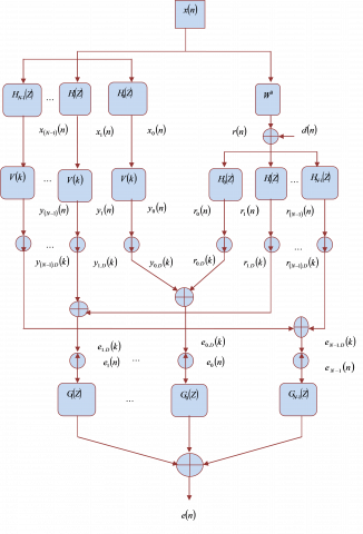
Context of NSAF: Both the optimal and resultant signals are partitioned into $N$ subbands, offered by $r_{i}(n)$ and $y_{i}(n)$ $i=0,1, \ldots, N-1 .$ The studied filters for these signals are described as $H_{0}(z), \ldots, H_{N-1}(z)$ that is indicated as in Figure 1
Figure 1. Overall architecture of NSAF
The signals of subband are allotted with corresponding bandwidth and are translated to the lower rate of sampling. In this technique, the actual sequences are represented as $n$ and $k$ which denotes the sequences that are evaluated. The decimated resultant signal for all subband signals is provided in Eq.(12), in which, $X_{i}(k)$ is assigned with $1 \times W$ row vector. Therefore, Eq.(3) is formulated as in Eq. (13). For determining $V^{o}$ with length $V$ Eq.(14) has been designed. The Eq.(15) and Eq. (16) can be employed to find out the fault signal of the devastated subband, in which, $r_{i, D}(k)=r_{i}(k N)$ indicates the essential signal which is decimated in the entire subbands. Hence, the NSAF filter is provided as in Eq. (17) in which the step-size is indicated by $\mu$.
$y_{i, D}(k)=Y_{i}(k) V(k)$ (12)
$Y_{i}(k)=\left[x_{i}(k N), x_{i}(k N-1) \ldots, x_{i}(k N-W+1)\right]$ (13)
$V(k)=\left[v_{o}(k), v_{1}(k), \ldots, v_{W-1}(k)\right]^{T}$ (14)
$e_{i, D}(k)=r_{i, D}(k)-y_{i, D}(k)$ (15)
$e_{i, D}(k)=r_{i, D}(k)-Y_{i}(k) V(k)$ (16)
$V(k+1)=V(k)+\mu \sum_{i=0}^{N-1} \frac{Y_{i}^{T}(k)}{\left\|Y_{i}(k)\right\|^{2}} e_{i, D}(k)$ (17)
4.2 Optimal subband selection for NSAF
The updating model for variation in step-size and required subband of the proposed NSAF filter is indicated as in Eq.(18), in which, $\gamma$ is bounded by error that is set to 1 for the conventional subbands and NSAFs that are chosen for matrix are represented by $U_{T_{M}} .$ On employing the directional factors and the step-size sequence $\left\{\mu_{k}\right\}$, the improvements in the SMNLMS indicate the convergence at zero as given in Eq.(19). As the magnitude is lesser than
of the predicted error, Eq. (20) is achieved.${{\hat{V}}_{M}}\left( k+1 \right)\,=\,\hat{V}\left( k \right)+\left\{ \begin{matrix} 1-\frac{\gamma }{\left| {{e}_{i}}\left( k \right) \right|}Y\left( k \right)\tilde{Y}{{U}_{{{T}_{M}}}}e\left( k \right);\,if\,\left| {{e}_{i}}\left( k \right) \right|>\gamma \\ 0;\,\,otherwise \\\end{matrix}\, \right.$ (18)
In Eq. (19) and Eq. (20), the index of time is represented by $k$ and it has the capacity to reveal the entire instance of timing owing to Eq. (21).
$\lim _{k \rightarrow \infty}\left\|\hat{V}_{k}-\hat{V}_{k-1}\right\|=\lim _{k \rightarrow \infty} \mu_{k}=0$ (19)
$\limsup _{k \rightarrow \infty}\left\|e_{i}(k)\right\| \leq \gamma$ (20)
$\left\|\hat{V}_{k}-\hat{V}_{k-1}\right\|=\mu_{k}=0$ otherwise (21)
As the spheroid $U_{n}$ is filled for the entire $k, \sigma_{k}^{2}>0 . \sigma_{k}^{2}$ is usually monotonic and therefore the sequence $\left\{\sigma_{k}^{2}\right\}$ is convergent. Depending on Eq. $(8),$ it can be assumed as given in Eq. (22) and Eq. (23)
$\frac{\mu_{k}^{2}\left\|e_{i}(k)\right\|^{2}}{\left\|x_{k}\right\|^{2}} \rightarrow 0$ (22)
$\left\|\hat{V}_{k}-\hat{V}_{k-1}\right\|=\frac{\mu_{k}\left\|e_{i}(k)\right\|}{\left\|x_{k}\right\|} \rightarrow 0$ (23)
Let us predict that, $\left\|x_{k}\right\|$ is bordered and method of updating are made by employing $\left\|e_{i}(k)\right\|>\gamma>0 .$ It is based upon $\mu_{k} \rightarrow 0 .$ Depending on Eq. $(11),\left\|e_{i}(k)\right\| \rightarrow \gamma$ is explained during the course of updating and $\|e(k)\|<$ \gammaotherwise, by which Eq. (18) is generated. The NSAFdependent updating design by means of subband assortment matrix $U_{T_{M}}$ is offered in Eq. (24).
$\hat{V}(k+1)=\hat{V}(k)+\mu_{i}(k) X(k)\left(Y^{T}(k) Y(k)\right)^{-1} U_{T_{N}} e(n)$ (24)
Greater correlation is achieved among $Y_{i}(k)$ with $\mu_{i}$ and thus the achieved formula is provided in Eq. (25) that is made easier to attain the modified design is as explained in Eq. (26) On the basis of the obtained error, $\mu$ is varied as in Eq. (27) and accordingly, the design is achieved as given in Eq. (27).
$\left\|\hat{V}_{M}(k+1)-\hat{V}(k)\right\|^{2}=\mu_{i}^{2}\left(Y^{T}(k) Y(k)\right)^{-1} e^{T}(n) U_{T_{N}} e(n)$ (25)
$\hat{V}_{M}(k+1)=\hat{V}(k)+\mu_{i}(k) Y(k) \widetilde{Y} U_{T_{N}} e(k)$ (26)
$\mu=\left\{\begin{array}{c}1-\frac{\gamma}{| e_{i}(k)} ; \text {if}\left|e_{i}(k)\right|>\gamma \\ 0 ; \text { otherwise }\end{array}\right.$ (27)
4.3 Determination of error bound and memorizing error
The error bound indicated by $\gamma$ is kept stable by employing Eq. (9), where the NSAF filter permits it to differ depending on the position of iteration. The proposed one to signify the error bound assessment is offered by Eq. (28). In Eq. (28), the present iteration is indicated by $k$ and $k_{\max }$ indicates the utmost iterations scheduled. The expression $\gamma\left(\gamma \max _{\min }\right)$ is the maximum and minimum error bounds, correspondingly.
$\gamma(k+1)=\gamma_{\min }+\frac{\left(\gamma_{\max }-\gamma_{\min }\right)(k+1)}{k_{\max }}$ (28)
Moreover, the error can be predicted depending on the variation among the real output and optimal output as in Eq. (15) and Eq. (16). As, the error is memorized till the preceding iteration, as in Eq. (29), the MVS-SNSAF regards the preceding error and standard existing error.
$e_{i, D}^{M}(k)=\frac{\left[r_{i, D}(k)-Y_{i}(k) V(k)\right]+e_{i, D}(k-1)}{2}$ (29)
As, the AF produces output by increasing a particular factor of weight with the input; it exists as a demanding one to consider the relevant weight, such that improved filtering can be achieved. In the traditional technique, the initialization is made by taking into account the amount of zeros in the echo cancellation system. Further, initialization in the implemented D-MVS-SNSAF technique is done depending on the description of the echo cancellation system. Consequently, the echo cancellation system can obtain better convergence.
Figure 2. Example of a echo cancellation system showing transition features
Assume an echo cancellation system with an input $x$ and output $\hat{r} .$ By means of the D-MVS-SNSAF model, weight for consistent echo cancellation system identification can be initialized for recognizing the polynomial design. This design can be explained by verifying the amount of transitions that happen in the output and input descriptions of the echo cancellation system as shown in Figure 2. According to Figure 2, almost ten transitions are displayed. Likewise, on the basis of output and input features, inconsistent transitions for all echo cancellation system can be achieved.
The conversions in the input-output features are exploited for describing the polynomial order. For enumerating the polynomial equation, primarily, the amount of orders and the amount of transitions have to be addressed.
$N^{\text {orders }}=N^{\text {transition } s}+1$ (30)
Accordingly, the amount of orders can be explained by taking into account the amount of conversions as in Eq. (30) in which $N^{\text {orders }}$ denotes the amount of orders and $N^{\text {transitions}}$ represents the amount of conversions in the input-output features.
On the whole, the conversions of the curves in input-output features can be categorized into six classifications namely, high to low, low to high, high to stable, low to stable, stable to low and stable to high that is offered by Eq. (31), Eq. (32), Eq. (33), Eq. (34), Eq. (35) and Eq. (36). Consequently, the polynomial formula can be explained by means of Eq. $(37),$ in which, $\hat{r}$ denotes the output of echo cancellation system. From Eq. (21) to $(36), \hat{r}(n-1)$ represents the preceding output of echo cancellation system, $\hat{r}(n)$ specifies the present output and $\hat{r}(n+1)$ denotes the subsequent output of echo cancellation system.
$\hat{r}(n-1)>\hat{r}(n)<\hat{r}(n+1)$ (31)
$\hat{r}(n-1)<\hat{r}(n)>\hat{r}(n+1)$ (32)
$\hat{r}(n-1)>\hat{r}(n)=\hat{r}(n+1)$ (33)
$\hat{r}(n-1)<\hat{r}(n)=\hat{r}(n+1)$ (34)
$\hat{r}(n-1)=\hat{r}(n)>\hat{r}(n+1)$ (35)
$\hat{r}(n-1)=\hat{r}(n)<\hat{r}(n+1)$ (36)
$\hat{r}=a_{0}+a_{1} x+a_{2} x^{2}+\ldots+a_{N^{\text {orders }}} x^{N^{\text {orders }}}$ (37)
For describing the initial weighting factor, the entire coefficients in Eq. (37) have to be resolved. Based on the whole coefficients, initialization of weighting factor takes place. As a result, the initial weight $(\left.V^{0}=V(k=0)\right)$ of the echo cancellation system is offered as given in Eq. (38). Moreover, the updating of weight is done by means of Eq. (9). Consequently, the improved system identification using echo cancellation technique can be achieved by appropriate initialization of weight by means of implemented D-MVS-SNSAF scheme and suitable update.
$V^{0}=\sum_{i=0}^{N} a_{i}$ (38)
6.1 Procedure
The proposed D-MVS-SNSAF for identifying echo cancellation system is simulated in MATLAB, and the experimental outcomes are distinguished with the traditional NSAF [4], SS-NSAF [32], VS-NSAF [21], VS-SNSAF [33] and MVS-SNSAF [34]. Here, two audio signals are used for experimentation. Moreover, the quantity of subbands adopted in VS-NSAF and NSAF is varied by 2, 4 and 8 to produce improved results. The considered mechanisms are executed for 1000 iterations when it is reciprocated for its up-sampling rate, and the down-sampling rate is set to 50%. The NSAF and SS-NSAF are allocated with a step-size 1. The implementation is done in the frequency of 384 Hz for the audio signal 1 and 215 Hz for the audio signal 2. The weight is measured for the non-determined echo cancellation systems by exploiting NSAF algorithms. As noise spoils the real echo cancellation systems, complications of the methods to lessen the noise are noted by varying the SNR of the input signal from 0 dB to 25 dB. The accomplished results are observed based on convergence analysis, error analysis, and stability analysis. In addition, the complications of the algorithm in minimizing noise are also examined in the forthcoming sections.
6.2 Error analysis: Converging behaviour
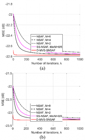
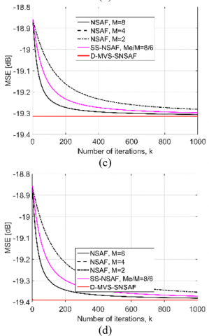
Figure 3. Convergence analysis on identification of echo cancellation system with respect to number of iterations without varying step-size (a) Audio signal 1 with order 1(b) Audio signal 1 with order 2 (c) Audio signal 2 with order 1 (d) Audio signal 2 with order 2
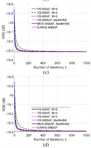
Figure 4. Convergence analysis on identification of echo cancellation system with respect to number of iterations with varying step-size (a) Audio signal 1 with order 1(b) Audio signal 1 with order 2 (c) Audio signal 2 with order 1 (d) Audio signal 2 with order 2
The convergence analysis for the proposed method on identification of echo cancellation system for two audio signals with respect to number of iterations for SNR at 25dB without varying step-size is given by Figure 3. Similarly, the audio signal 1 for order 1is given by Figure 3(a), where the proposed method is 3.9 % superior to NSAF with 8 subbands, 1.27 % superior to NSAF with 2 subbands and 0.6 % superior to SS-NSAF for 200th iteration. From Figure 3(b), the audio signal 1 for order 2 is obtained in which the proposed method for 200th iteration is 0.2 % superior to NSAF with 8 subbands, 2.3 % superior to NSAF with 2 subbands and 0.6 % superior to SS-NSAF techniques. Also, from Figure 3(c), in the audio signal 2 for order 1, for 800th iteration, the implemented technique is 0.15 % better than NSAF with 8 subbands, 3.6 % better than NSAF with 2 subbands and 3.1 % better than SS-NSAF methods. Similarly, from Figure 3(d), the audio signal 2 for order 2, the implemented technique is 0.2 % better than NSAF with 8 subbands, 0.8 % better than NSAF with 2 subbands and 0.46 % better than SS-NSAF techniques for 200th iteration. Thus, the capability of the proposed method is verified.
The convergence analysis for the implemented scheme on system identification with respect to number of iterations with varying step-size is given by Figure 4. Similarly, the audio signal 1 for order 1is given by Figure 4(a), where the proposed method at 25 dB for 200th iteration is 3.9% superior to VS-NSAF with 8 subbands and VS-NSAF with 4 subbands, 0.6 % superior to VS-NSAF with 2 subbands, 3.9 % superior to MVS-SNSAF respectively. From Figure 4(b), the audio signal 1 for order 2 is obtained in which the proposed method for 200th iteration is 0.8 % superior to VS-NSAF with 2 subbands, 0.42 % superior to VS-NSAF with 4 subbands and 0.42 % superior to MVS-SNSAF techniques at 25 dB. Also, from Figure 4(c), in the audio signal 2 for order 1, the implemented technique for 400th iteration is 1 % better than all other compared techniques at 25 dB. Similarly, from Figure 4(d), the audio signal 2 for order 2, the implemented technique for 800th iteration is 5 % superior to all other distinguished techniques at 25 dB. Thus the capacity of the implemented technique in identifying echo cancellation system is validated.
6.3 Noise effect
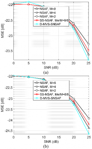
The error convergence analysis on identification of echo cancellation system at different SNR without varying step-size is given by Figure 5. Similarly, from Figure 5(a) the audio signal 1 for order 1is shown in which the implemented technique is 2.9 % superior to NSAF with 2 subbands, 1.6 % superior to NSAF with 8 subbands and 2 % superior to SS-NSAF methods at 25 dB. Also, from Figure 5(b), in the audio signal 1 for order 2, the proposed method is 0.8 % better than NSAF with 8 subbands, 2.4 % better than NSAF with 2 subbands and 1.2 % better than SS-NSAF methods at 25 dB. From Figure 5(c), from the audio signal 2 for order 1, the implemented technique is 0.9 % superior to NSAF with 8 subbands, 2.4 % superior to NSAF with 2 subbands and 1.4 % superior to SS-NSAF methods at 25 dB. Moreover, from Fig. 5(d), the audio signal 2 for order 2, the proposed technique is 2.4 % better than NSAF with 2 subbands, 0.49 % better than NSAF with 8 subbands and 0.9 % better than SS-NSAF methods at 25 dB respectively. Thus, the error minimizing capability of the implemented scheme is verified.
Figure 5. Error minimization with respect to SNR without varying step-size (a) Audio signal 1 with order 1(b) Audio signal 1 with order 2 (c) Audio signal 2 with order 1 (d) Audio signal 2 with order 2
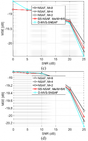
Figure 6. Error minimization with respect to SNR with varying step-size (a) Audio signal 1 with order 1(b) Audio signal 1 with order 2 (c) Audio signal 2 with order 1 (d) Audio signal 2 with order 2
The error convergence analysis on identification of echo cancellation system at different SNR with varying step-size is given by Figure 6. Similarly, from Figure 6(a), the audio signal 1 for order 1 is shown in which the implemented technique is 0.83 % superior to all the compared methods at 25 dB. Also, from Figure 6(b), in the audio signal 1 for order 2, the proposed method is 4.66 % better than the entire distinguished methods. From Figure 6(c), in the audio signal 2 for order 1, the implemented technique at 25 dB is 0.51 % superior to all other compared methods. Moreover, from Figure 6(d), in the audio signal 2 for order 2, the proposed technique at 25 dB is 0.98 % better than the entire compared techniques. Thus, the error reducing capability of the proposed echo cancellation system with varying step-size is explained.
6.4 Stability analysis
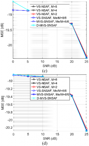
Figure 7(a) and Figure 7(b) shows the comparison of stability between proposed D-MVS-SNSAF algorithm and conventional methods for audio signal 1 and audio signal 2 in terms of step-size. From the analysis, it can be observed that the proposed method achieves better step-size with minimum number of iterations, while other algorithms attain high step-size with increased number of iterations. Thus, the proposed algorithm shows better stability analysis when compared with other algorithms.
Figure 7. Stability analysis on echo cancellation system identification with respect to number of iterations (a) Audio signal 1 (b) Audio signal 2
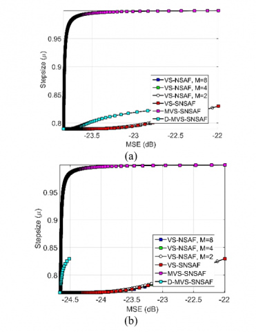
Figure 8. Evaluation of step-size on echo cancellation system identification with respect to to MSE (a) Audio signal 1 (b) Audio signal 2
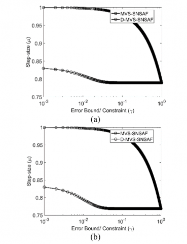
Figure 9. Estimation of step-size on identification of echo cancellation system with respect to error bound constraints (a) Audio signal 1 (b) Audio signal 2
Figure 8(a) and Figure 8(b) shows the comparison of step-size with respect to MSE for the proposed D-MVS-SNSAF algorithm and conventional methods for audio signal 1 and audio signal 2 in terms of step-size. From Figure 8(a) and Figure 8(b), it can be seen that the implemented method acquires higher step-size with minimized error rate, while other methods attain maximum step-size with increase in error rate. Thus, the improved performance of the proposed method is revealed. Similarly, Figure 9 shows the evaluation of step-size on identification of echo cancellation system with respect to error bound constraints. From Figure 9(a) and Figure 9(b), it can be noted that the implemented D-MVS-SNSAF algorithm obtains maximum step-size with minimum error rate. On the other hand, the compared method attains a maximum step-size with increase in error rate. Hence, it can be concluded that the proposed mechanism offers better performance capability when compared with the existing techniques.
This paper has presented improvements in identifying the echo cancellation systems by exploiting an enhanced NSAF technique said to be the D-MVS-SNSAF method. According to this technique, the number of transitions in the input/output signals was measured for deriving the polynomial from two audio signals as input. Following the simulation, the proposed D-MVS-SNSAF method was compared with the existing techniques such as NSAF, VS-NSAF, SS-NSAF VS-SNSAF and MVS-SNSAF methods. From the analysis, it was observed that the convergence analysis of the proposed method is 3.9 % superior to VS-NSAF with 8 subbands and VS-NSAF with 4 subbands, 0.6 % superior to VS-NSAF with 2 subbands, 3.9 % superior to MVS-SNSAF techniques respectively. Also, the error convergence analysis of the implemented technique was 2.9% superior to NSAF with 2 subbands, 1.6 % superior to NSAF with 8 subbands and 2 % superior to SS-NSAF methods at 25 dB techniques. Moreover, the proposed method has delivered better results in terms of stability. Thus on the basis of achieved results, the computational improvements of the implemented D-MVS-SNSAF method were revealed.
|
Acronym |
Description |
|
AF |
Adaptive Filter |
|
SAF |
Subband Adaptive Filter |
|
AEC |
Acoustic echo cancellation |
|
NSAF |
Normalized subband Adaptive Filter |
|
LMS |
Least mean square |
|
NLMS |
Normalized least mean square |
|
SEP |
Sparse Echo Paths |
|
VSS |
Variable step-size |
|
SM-NSAF |
Set-membership NSAF |
|
PNSAF |
Proportionate NSAF |
|
MPNSAF |
$\mu$ law PNSAF |
|
SS-MSE |
Steady-state mean square Error |
|
SSMS |
Steady-State Mean Square |
|
SSE |
Steady-State Error |
|
RSM |
Robust Set Membership |
|
RSM-NSAF |
Robust set membership NSAF |
|
SM-NSAF |
Set-membership NSAF |
|
SSAF |
Sign SAF |
|
APA |
Affine projection algorithm |
|
VSSM-NSAF |
Variable step-size matrix NSAF |
|
RVSS-NSAF. |
Robust variable step-size NSAF |
|
CIPNSAF |
Combined improved PNSAF |
|
APSAF |
Affine projection subbandAF |
|
VS-SNSAF |
Variable Step-size based NSAF with Selected subbands |
|
VS-NSAF |
Variable Step-size NSAF |
|
SS-NSAF |
Selective Subbands NSAF |
|
MVS-SNSAF |
Memorized error and varying error bound Variable Step-size based NSAF with Selected subbands |
|
SNR |
Signal to Noise Ratio |
|
CNSAF |
Combined NSAF |
|
FIR |
Finite Impulse Response |
|
D-MVS-SNSAF |
Deterministic Initialization-based MVS-SNSAF |
[1] Yu, Y., Zhao, H. (2017). Proportionate normalized subband adaptive filter algorithms with sparseness-measured for acoustic echo cancellation. AEU-International Journal of Electronics and Communications, 75: 53-62. https://doi.org/10.1016/j.aeue.2017.03.009
[2] Zheng, Z., Liu, Z., Zhao, H., Yu, Y., Lu, L. (2017). Robust set-membership normalized subband adaptive filtering algorithms and their application to acoustic echo cancellation. IEEE Journals & Magazines, 64(8): 2098–2111. https://doi.org/10.1109/TCSI.2017.2685679
[3] Ni, J., Li, F. (2010). Adaptive combination of subband Adaptive Filters for acoustic echo cancellation. IEEE Journals & Magazines, 56(3): 1549–1555. https://doi.org/10.1109/TCE.2010.5606296
[4] Yu, Y., Zhao, H., He, Z., Chen, B. (2016). A robust band-dependent variable step-size normalized subband adaptive filter algorithm against impulsive noises. Signal Processing, 119: 203-208. https://doi.org/10.1016/j.sigpro.2015.07.028
[5] Yu, Y., Zhao, H. (2016). Adaptive combination of proportionate normalized subband adaptive filter with the tap-weights feedback for acoustic echo cancellation. Wireless Pers Communications, 92(2): 467-481. https://doi.org/10.1007/s11277-016-3552-x.
[6] Petraglia, M.R., Haddad, D.B., Marques, E.L. (2016). Affine projection subband AF with low computational complexity. IEEE Journals & Magazines, 63(10): 989-993. https://doi.org/10.1109/TCSII.2016.2539080
[7] Ni, J., Li, F. (2010). A variable step-size matrix normalized subband adaptive filtering. IEEE Journals & Magazines, 18(6): 1290-1299. https://doi.org/10.1109/TASL.2009.2032948
[8] Yu, Y., Zhao, H. (2017). Proportionate normalized subband adaptive filter algorithms with sparseness-measured for acoustic echo cancellation. AEU - International Journal of Electronics and Communications, 75: 53-62. https://doi.org/10.1016/j.aeue.2017.03.009
[9] Jain, A., Goel, S., Nathwani, K., Hegde, R.M. (2015). Robust acoustic echo cancellation using Kalman filter in double talk scenario. Speech Communication, 70: 65-75. https://doi.org/10.1016/j.specom.2015.03.002
[10] Schüldt, C., Lindstrom, F., Li, H., Claesson, I. (2009). Adaptive filter length selection for acoustic echo cancellation. Signal Processing, 89(6): 1185-1194. https://doi.org/10.1016/j.sigpro.2008.12.023
[11] Stanciu, C., Benesty, J., Paleologu, C., Gänsler, T., Ciochină, S. (2013). A widely linear model for stereophonic acoustic echo cancellation. Signal Processing, 93(2): 511-516. https://doi.org/10.1016/j.sigpro.2012.08.017
[12] Kuech, F., Kellermann, W. (2006). Orthogonalized power filters for nonlinear acoustic echo cancellation. Signal Processing, 86(6): 1168-1181. https://doi.org/10.1016/j.sigpro.2005.09.014
[13] Contan, C., Kirei, B.S., T¸opa, M.D. (2013). Modified NLMF adaptation of Volterra filters used for nonlinear acoustic echo cancellation. Signal Processing, 93(5): 1152-1161. https://doi.org/10.1016/j.sigpro.2012.11.017
[14] Cecchi, S., Romoli, L., Peretti, P., Piazza, F. (2012). Low-complexity implementation of a real-time decorrelation algorithm for stereophonic acoustic echo cancellation. Signal Processing, 92(11): 2668-2675. https://doi.org/10.1016/j.sigpro.2012.04.013
[15] Özbay, Y., Kavsaoğlu, A.R. (2010). An optimum algorithm for adaptive filtering on acoustic echo cancellation using TMS320C6713 DSP. Digital Signal Processing, 20(1): 133-148. https://doi.org/10.1016/j.dsp.2009.05.001
[16] Ma, B., Dong, H., Zhu, Y. (2011). An improved subband adaptive filtering for acoustic echo cancellation application. Procedia Engineering, 15: 2244-2249. https://doi.org/10.1016/j.proeng.2011.08.420
[17] Shi, K., Ma, X., Zhou, G.T. (2009). An efficient acoustic echo cancellation design for systems with long room impulses and nonlinear loudspeakers. Signal Processing, 89(2): 121-132. https://doi.org/10.1016/j.sigpro.2008.07.009
[18] Mader, A., Puder, H., Schmidt, G.U. (2000). Step-size control for acoustic echo cancellation filters – an overview. Signal Processing, 80(9): 1697-1719. https://doi.org/10.1016/S0165-1684(00)00082-7
[19] Tahernezhadi, M., Liu, J. (1997). A subband approach to adaptive acoustic echo cancellation. Computers & Electrical Engineering, 23(4): 205-215. https://doi.org/10.1016/S0045-7906(97)00011-6
[20] Chen, K., Xu, P., Lu, J., Xu, B. (2009). An improved post-filter of acoustic echo canceller based on subband implementation. Applied Acoustics, 70(6): 886-893. https://doi.org/10.1016/j.apacoust.2008.10.004
[21] Wen, P., Zhang, J. (2017). A novel variable step-size normalized subband adaptive filtering based on mixed error cost function. Signal Processing, 138: 48-52. https://doi.org/10.1016/j.sigpro.2017.01.023
[22] Wen, P., Zhang, J. (2017). Robust variable step-size sign subband adaptive filtering algorithm against impulsive noise. Signal Processing, 139: 110-115. https://doi.org/10.1016/j.sigpro.2017.04.012
[23] Yu, Y., Zhao, H. (2017). Performance analysis of the deficient length Normalized subband Adaptive Filter algorithm and a variable step-size method for improving its performance. Digital Signal Processing, 62: 157-167. https://doi.org/10.1016/j.dsp.2016.11.009
[24] Choi, Y. (2014). A new subband adaptive filtering algorithm for sparse system identification with impulsive noise. Journal of Applied Mathematics 2014, Article ID 704231, 1-7. https://doi.org/10.1155/2014/704231
[25] Yu, Y., Zhao, H. (2018). Robust incremental normalized least mean square algorithm with variable step-sizes over distributed networks. Signal Processing, 144: 1-6. https://doi.org/10.1016/j.sigpro.2017.09.016
[26] Cho, H., Lee, C.W., Kim, S.W. (2009). Derivation of a new normalized least mean squares algorithm with modified minimization criterion. Signal Processing, 89(4): 692-695. https://doi.org/10.1016/j.sigpro.2008.10.026
[27] Abadi, M.S.E., Husøy, J.H. (2008). Selective partial update and set-membership subband adaptive filters. Signal Processing, 88(10): 2463-2471. https://doi.org/10.1016/j.sigpro.2008.04.014
[28] Ni, J., Chen, X. (2013). Steady-state mean-square error analysis of regularized normalized subband adaptive filters. Signal Processing, 93(9): 2648-2652. https://doi.org/10.1016/j.sigpro.2013.03.030
[29] Kechichian, P., Champagne, B. (2009). An improved partial haar dual adaptive filters for rapid identification of a sparse echo channel. Signal Processing, 89(5): 710-723. https://doi.org/10.1016/j.sigpro.2008.10.033
[30] Darlington, D.J., Campbell, D.R. (1996). Subband, dual-channel adaptive noise cancellation using normalised LMS. IEEE Conference Publications, 1996 8th European Signal Processing Conference (EUSIPCO 1996), 1–4. https://doi.org/10.1109/DSPWS.1996.555527
[31] Christelle, Y.T. (2013). Acoustic echo cancellation for single- and dual-microphone devices: Application to mobile devices. Networking and Internet Architecture [cs.NI]. Télécom ParisTech.
[32] Song, M., Kim, S., Choi, Y., Song, W. (2013). Selective normalized subband adaptive filtering with subband extension. IEEE Transactions on Circuits and Systems II: Express Briefs, 60(2): 101-105. https://doi.org/10.1109/TCSII.2012.2235737
[33] Samuyelu, B., Rajesh Kumar, P. (2017). Normalised subband adaptive filtering with extended adaptiveness on degree of subband filters. International Journal of Electronics, 104(12): 2048-2061. https://doi.org/10.1080/00207217.2017.1335792
[34] Samuyelu, B., Rajesh Kumar, P. (2018). Error memory and varying error bound for extending adaptiveness for normalized subband adaptive filtering. Alexandria Engineering Journal, 57(4): 2445-2453. https://doi.org/10.1016/j.aej.2017.08.005