Rahmouna Cheriet* | Bourassia Bensaad | Fatiha Bouhadjela | Soufyane Belhenini | Mohammed Belharizi
© 2021 IIETA. This article is published by IIETA and is licensed under the CC BY 4.0 license (http://creativecommons.org/licenses/by/4.0/).
OPEN ACCESS
This study presents a mixed numerical / semi-empirical approach that primarily aimed to estimate the thermal contact resistance between two solids. The results obtained by this mixed method were compared and validated by experimental measurements of this resistance. Three semi-empirical models were used, namely the Mikic model, the Yovanovich model and the Antonetti model. The three-dimensional finite element numerical simulation was used to estimate the contact pressure between the two solids. Then this contact pressure obtained numerically was compared to the hardness of the solids in contact. The findings indicated that the numerically obtained contact pressures were close to hardness. Therefore, the hardness, which is usually used as an input variable in semi-empirical models, was replaced by the contact pressure. The thermal contact resistance obtained by this mixed method was then compared with the experimental one. The outcomes obtained from this comparison turned out to be very conclusive and can therefore be used to reinforce our approach which can actually be viewed as a reliable and low-cost method for estimating the thermal contact resistance between solids in contact.
thermal contact resistance, hardness, semi-empirical models, actual contact rate, contact pressure, finite elements
The thermal contact resistance (TCR) is an essential property for the modeling of structures involving materials in contact. Indeed, when two solids are in contact, due to the roughness and non-flatness of their surfaces, the contact never takes place over the entire apparent surface, but only in certain zones [1, 2]. Most metal surfaces make up only a small portion of about 1 to 2% [3] of the apparent contact area [4, 5]. These zones are located on the asperity peaks of the surfaces, which engenders the phenomenon of thermal contact resistance (TCR) [2]. It should be noted that the TCR has been widely studied theoretically and experimentally. The experimental measurements of TCR require specific means and necessitate a lot of time to prepare samples, perform measurements, analyze results, etc. Several semi-empirical models for the estimation of the thermal contact resistance have been reported in the literature [6-12]. These models require knowledge of a number of parameters, including hardness, to be used in formulas of semi-empirical models studied in this article, and consequently, a number of experiments will have to be carried out again. In order to circumvent these difficulties which involves the use of experimentation, it was deemed necessary to use a mixed approach.
For this, many numerical models were developed by the finite element method (FEM) in order to estimate the contact pressure between two solids (sapphire / brass) in contact. The contact pressures obtained were then compared to the hardness of the materials under study. Afterwards, the contact pressures obtained numerically were used as input variables in semi-empirical models [10-12] instead of hardness. This choice is supported by the hypothesis of Abbott and Firstone [13]. These same models were used to estimate the TCR which in turn was compared to the TCR measured experimentally [14, 15].
2.1 Determination of the thermal contact resistance
Figure 1 (a) shows that, on a microscopic scale, contact between two solids is not totally perfect. Figure 1 (b) illustrates the phenomenon of constriction of the flow lines at the contact. TCR is the equivalent resistance of two parallel resistance Rs and Rf characterizing respectively the heat transfer through the "solid- solid" path and the heat transfer through the "solid-fluid-solid" path [16, 17]. The thermal contact resistance is given as follows:
$\mathrm{TCR}=\frac{\text { Rs. Rf }}{\mathbf{R s}+\mathbf{R f}}$ (1)
where,
$\mathbf{R f}=\frac{\mathbf{d}}{\lambda_{\mathbf{f}}}$ (2)
where,
Figure 1. Interface diagram at the microscopic contact level
2.2 Presentation of semi-empirical models
Among the numerous semi-empirical models for the estimation of TCR found in the literature, three of the best-known ones were selected: the Mikic [10] model, the Yovanovich [11] model and the Antonetti et al. [12] model. These three models are based on the one previously developed by Cooper et al. [18]. This model expresses the constriction resistance in the form of the following equation:
$R s=\frac{1}{c 1} \cdot \frac{\sigma}{m \lambda_{s}} \cdot\left(\frac{H_{v}}{p}\right)^{c 2}$ (3)
where,
$\lambda_{s}=\frac{2 \lambda_{1} \cdot \lambda_{2}}{\lambda_{1}+\lambda_{2}} \approx 59$, with $\lambda_{1}=115, \lambda_{2}=40$
2.2.1 The Mikic model
Mikic [10] proposed several analytical expressions for the thermal contact resistance while taking into account the case of plastic or elastic deformations. In the case of plastic deformation, for low loads with a plasticity coefficient varying between 0.9 and 1.3 and a deformation of asperities between 50 and 90% of the contact surface, the thermal contact resistance may be calculated as follows:
$R s=\frac{\mathbf{1}}{\mathbf{1}, \mathbf{1} \mathbf{3}} \cdot \frac{\boldsymbol{\sigma}}{\boldsymbol{m} \lambda_{s}}$ (4)
However, in the case of heavy loads with a coefficient of plasticity equal to 2.5 and the deformation of asperities remains elastic as long as the contact surface is less than 0.1%, the thermal contact resistance can be evaluated using the expression:
$R s=\frac{\mathbf{1}}{\mathbf{1}, \mathbf{1 3}} \cdot \frac{\boldsymbol{\sigma}}{\boldsymbol{m} \lambda_{s}} \cdot\left(\frac{\boldsymbol{p}+\boldsymbol{H}_{v}}{p}\right)^{\mathbf{0 , 9 4}}$ (5)
2.2.2 The Yovanovich model
This model [11] expresses the constriction resistance for a plastic deformation as follows:
$R s=\frac{1}{1,25} \cdot \frac{\sigma}{m \lambda_{s}} \cdot\left(\frac{H_{c}}{p}\right)^{0,95}$ (6)
where,
2.2.3 The Antonetti model
Antonetti et al. [12] expressed the constriction resistance for a plastic deformation as a function of the surface parameters in the following form:
$R s=\frac{1}{35,33 \cdot \lambda_{s}} \cdot R_{a}^{0,598}\left(\frac{H_{v}}{p}\right)^{0,95}$ (7)
where,
Three-dimensional numerical models, using the ANSYS finite element analysis computer software program, were applied to estimate the contact pressure between the two solids (sapphire / brass) under study. The numerically obtained contact pressure would then be used in place of hardness in semi-empirical formulas for the purpose of estimating the thermal contact resistance.
3.1 Geometry
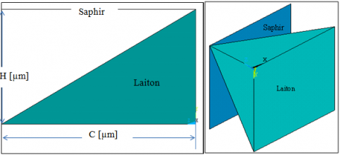
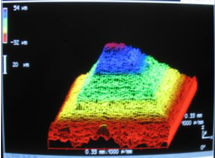
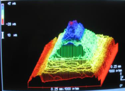
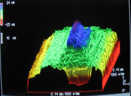
Figure 2 illustrates the contact between a smooth and rigid sapphire plane and a deformable pyramidal brass asperity. In accordance with the experimental measurements depicted in Figure 3, three sizes of square-based pyramids PYR1in Figure 3 (b), PYR2 in Figure 3 (c) and PYR3 in Figure 3 (d), were selected. For the sake of rationalizing the costs of our calculations, it was deemed useful to exploit the existing symmetries. For this, only a quarter of the structure was modeled. The dimensions of the pyramidal asperities are presented in Table 1.
Figure 2. 2D and 3D geometric models
(a) Capture des 9 pyramides, exemple
(b) PYR 1
(c) PYR 2
(d) PYR 3
Figure 3. Survey of a 1 mm2 area on the three pyramidal surfaces [15]
Table 1. Dimensions of pyramidal asperities [15]
|
|
C(µm) |
H (µm) |
|
PYR 1 |
330 |
90 |
|
PYR 2 |
252 |
77 |
|
PYR 3 |
140 |
50 |
3.2 Boundary conditions and meshing
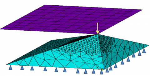
In this part, the model was supposed to be embedded at the base of the pyramid and a displacement between 2.5 and 17.5 µm was imposed on the rigid plane of this model (Figure 4). In addition, the solid element 187 was used for the meshing. The numerical model had 7120 elements for the case PYR 1, 5951 elements for the case PYR 2, and 4641 elements for the case PYR 3. This choice was made once the sensitivity to the mesh was achieved.
Figure 4. Boundary conditions and meshing
3.3 Properties of materials
Table 2 summarizes the mechanical properties of the materials studied. Besides, the characteristic elastoplastic curve of brass is given in Figure 5.
Figure 5. Stress-strain curve of brass [19]
Table 2. Properties of materials used [15]
|
|
E (GPa) |
ν |
|
brass |
97 |
0.35 |
|
sapphire |
440 |
0.3 |
4.1 Comparing the contact pressure estimated by numerical simulation and the experimental hardness
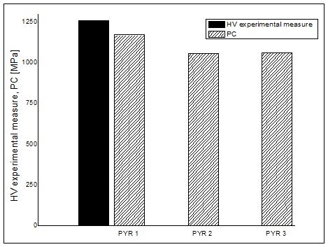
First, the contact pressure between the brass pyramidal asperity and the rigid plane was estimated. Then, the values obtained for the contact pressure were compared to the Vickers hardness of brass. Figure 6 clearly shows the results of the comparisons. One can easily note that the values of the contact pressures estimated numerically are close to the Vickers hardness measured experimentally. Hence, the case PYR1 exhibits a contact pressure 8% less than the hardness. However, for the two cases PYR 2 and PYR 3, that difference was around 17%. The average difference is about 13% which may be considered as acceptable. These findings allowed validating the numerical model in accordance with the Abbott and First one approach. It is consequently possible to use this numerical quantity (the contact pressure) in the semi-empirical models with a view to estimating the thermal contact resistance instead of the Vickers hardness.
Figure 6. Comparison between the contact pressure estimated numerically and the Vickers hardness measured experimentally
(a) PYR1 [19]
(b) PYR2
(c) PYR3
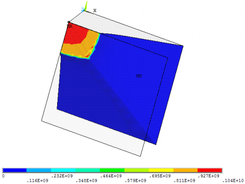
Figure 7. The actual contact pressure for the three geometric models under study
Figure 7 illustrates the zones of contact stress concentration. It is easy to see that the three models have the same zones of high pressure.
4.2 Comparing the experimental thermal contact resistance and that estimated with the mixed numerical / semi-empirical approach
The thermal contact resistance (TCR) values were calculated using the models described in the first part of the article, namely the Mikic model (high and low loads), the Yovanovich model and the Antonetti model. The geometric parameters introduced into these models are summarized in Table 3. The contact pressures obtained numerically were injected into the models instead of the hardness. The TCR values calculated by this approach were then compared with those measured experimentally. The comparison was carried out for each case separately.
4.2.1 Comparison for the case PYR1
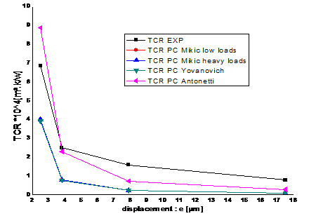
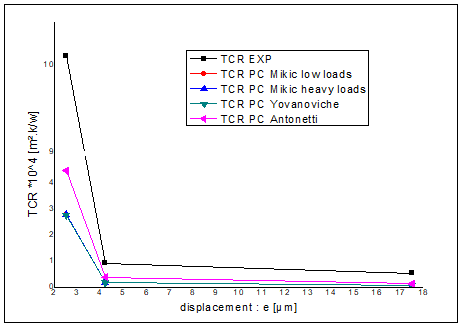
Figure 8 illustrates a comparison between the experimental TCR (TCR EXP) and that calculated by the mixed approach. The evolution of the TCR is given as a function of the imposed displacement. It was observed that the curves obtained by the mixed (numerical / semi-empirical) approach are nearly similar to that obtained experimentally. Moreover, the experimentally measured TCR remained above that estimated by the mixed approach. In addition, it should be noted that the mixed approach gave the same order of magnitude as the experimental method. It is worth mentioning that the mixed approach, using Antonetti's model, gave TCR values that are quite similar to those measured experimentally. The mixed approach using the Mikic and Yovanovich models allowed obtaining values that are close to each other.
Figure 8. Comparison between the TCR experimental values and those obtained by the mixed approach for the case PYR1
4.2.2 Comparison for the case PYR2
Figure 9 shows a comparison between the values of the experimental TCR (TCR EXP) values and those calculated with the mixed approach. It is clearly noted that the evolution of the experimental TCR as a function of the imposed displacements is comparable to that of the TCR obtained by the mixed approach as a function of the same displacements. It should also be noted that the mixed approach provided the same order of magnitude as the experimental method. The mixed approach, which is based on the Antonetti model, gave the TCR values closest to those measured experimentally.
Table 3. The geometric parameters of the three surfaces studied [15]
|
P (bars) |
PYR1 |
PYR 2 |
PYR 3 |
||||||
|
Ra (µm) |
Rq (µm) |
m |
Ra (µm) |
Rq (µm) |
m |
Ra (µm) |
Rq (µm) |
m |
|
|
2.5 |
16.1 |
19.5 |
1.28 |
11.5 |
14.1 |
0,61 |
5.25 |
7 |
0.66 |
|
20 |
16 |
19 |
11 |
14 |
- |
- |
|||
|
75 |
16.1 |
19.6 |
11.5 |
14.1 |
5.2 |
6.9 |
|||
|
215 |
16.05 |
19.4 |
11.5 |
14 |
5.2 |
6.9 |
|||
Figure 9. Comparison between the experimental TCR values and those obtained by the mixed approach for the case PYR2
Figure 10. Comparison between the experimental values and those obtained by the mixed approach for the case PYR3
4.2.3 Comparison for the case PYR3
Figure 10 presents a comparison between the experimental TCR (TCR EXP) values and those calculated with the mixed approach for the case PYR3. One may easily observe that the curves, the experimental and those obtained by our approach, follow the same pattern. The TCR values estimated by our approach are of the same order of magnitude as those measured experimentally. In addition, the mixed approach, which is based on the Antonetti model, gave TCR values closest to the experimental ones.
4.2.4 Comparison of the thermal contact resistances in the three cases
Figure 11 summarizes the comparisons for the three cases under study. The mixed approach, which is based on the Antonetti model, is the one that provided TCR values closest to those measured experimentally, whatever the case. It should be noted that the case PYR3 is the least precise of the three cases studied. The TCR values obtained by the mixed approach, which uses the Mikic and Yovanovich models, are very close to each other.
Figure 11. Comparison histogram of the mean TCR values measured experimentally and those estimated by our mixed approach for all three cases
A mixed numerical / semi-empirical approach was developed in order to estimate the thermal resistance of a solid-to-solid contact. This approach is based on semi-empirical models in which the input variables are determined by numerical finite element simulations. For this, three cases, i.e. PYR1, PYR2 and PYR3, were studied. The main results of the comparison between the thermal resistance values measured experimentally (TCR EXP) and those estimated by the mixed approach are summarized in the following points:
|
TCR |
Thermal contact resistance |
|
Rs |
Thermal contact resistance at the interface solid-solid (Resistance of Constriction) |
|
Rf |
Thermal contact resistance at the interface solid-fluid-solid |
|
d |
Separation distance between the median planes of the two surfaces in contact |
|
m |
Slope of the asperity |
|
Hv |
Vickers hardness |
|
Hc |
Effective hardness |
|
P |
Applied pressure |
|
Pc |
Contact Pressure |
|
Ra Rq |
Arithmetic roughness Quadratic roughness |
|
T |
Temperature |
|
E |
Young’s module |
|
c1,c2 |
Coefficients |
|
Symbols grec |
|
|
λf |
Thermal conductivity of air |
|
σ |
Quadratic roughness |
|
λs |
Equivalent thermal conductivity |
|
Indices |
|
|
s |
Solid |
|
f |
Fluid |
|
r |
Reel |
|
1 |
Solid 1 |
|
2 |
Solid 2 |
[1] Min, J.P., Jeong, K.M., Jaehoon, B., Young, K.J. (2020). Thermal contact conductance-based thermal behavior analytical model for a hybrid floor at elevated temperatures. Mater, 13: 1-16. https://doi.org/10.3390/ma13194257
[2] Chadouli, R., Frédéric, L., Iulian, R., Makhlouf, M. (2019). Numerical study of the surface roughness, thermal conductivity of the contact materials and interstitial fluid convection coefficient effect on the thermal contact conductance. Annales de Chimie - Science des Matériaux, 43(4): 265-271. https://doi.org/10.18280/acsm.430410
[3] Bardon. (1971). Introduction to the study of thermal contact resistance. Presented at French Society of Thermic. Poitiers.
[4] Archard, J.F. (1957). Elastic deformation and the lows of friction. Royal Society, 243(1233): 190-205. https://doi.org/10.1098/rspa.1957.0214
[5] Bowden, F.P., Tabor, D. (1954). The Friction and Lubrication of Solids. Clarendon Press. https://doi.org/10.1126/science.113.2938.443-a
[6] Singhal, V., Litke, P.J., Black, A.F., Garimella, S.V. (2005). An experimentally validated thermo-mechanical model for the prediction of thermal contact conductance. International Journal of Heat and Mass Transfer, 48(25-26): 5446-5459. https://doi.org/10.1016/j.ijheatmasstransfer.2005.06.028
[7] Sridhar, M.R., Yovanovich, M.M. (1996). Elastoplastic contact conductance model for isotropic conforming rough surfaces and comparison with experiments. Journal of Heat Transfer, 118(1): 3-9. https://doi.org/10.1115/1.2824065
[8] Antonetti, V.W., Yovanovich, M.M. (1985). Enhancement of thermal contact conductance by metallic coatings: Theory and experiment. Journal of Heat Transfer, 107(3): 513-519. https://doi.org/10.1115/1.3247454
[9] Yovanovich, M.M. (2005). Four decades of research on thermal contact, gap, and joint resistance in microelectronics. IEEE Transactions on Components and Packaging Technologies, 28(2): 182-206. https://doi.org/10.1109/TCAPT.2005.848483
[10] Mikić, B.B. (1974). Thermal contact conductance; theoretical considerations. International Journal of Heat and Mass Transfer, 17(2): 205-214. https://doi.org/10.1016/0017-9310(74)90082-9
[11] Yovanovich, M.M. (1986). Recent developments in thermal contact, gap and joint conductance theories and experiment. In Heat Transfer 1986; Proceedings of the Eighth International Conference, pp. 35-45. https://doi.org/10.1615/IHTC8.2260
[12] Antonetti, V.W., Whittle, T.D., Simon, R.E. (1993). An approximate thermal contact conductance correlation. Journal of Electronic Packaging, 115(1): 131-134. https://doi.org/10.1115/1.2909293
[13] Abbott, E.J., Firestone, F.A. (1995). Specifying surface quality: A method based on accurate measurement and comparison. Spie Milestone Series MS, 107: 63.
[14] Bourassia, B., Brahim, B. (2019). Analysis of the evolution of the structure of a surface with pyramidal asperities in contact with a hard and smooth plane. Journal of Heat Transfer, 142(1): 011401. https://doi.org/10.1115/1.4045303
[15] Bensaad, B. (2008). Experimental study of evolution and of establishment of the state of surface of a metallic material in contact with a plan of sapphire: Application has the modelling of the thermal resistance of contact. Polytechnic School of the University of Nantes.
[16] Guillermo, F.U., Diana, R., Domingo, A.T. (2021). Estimation of a thermal conductivity in a stationary heat transfer problem with a solid-solid interface. International Journal of Heat and Technology, 39(2): 337-344. https://doi.org/10.18280/ijht.390202
[17] Guillermo, F.U., Diana, R., Domingo, A.T. (2020). Estimation technique for a contact point between two materials in a stationary heat transfer problem. Mathematical Modelling of Engineering Problems, 7(4): 607-613. https://doi.org/10.18280/mmep.070413
[18] Cooper, M.G., Mikic, B.B., Yovanovich, M.M. (1969). Thermal contact conductance. International Journal of Heat and Mass Transfer, 12(3): 279-300. https://doi.org/10.1016/0017-9310(69)90011-8
[19] Bouhadjela, F., Bensaad, B., Cheriet, R., Belharizi, M., Belhenini, S. (2020). Contribution to the study of plastic mechanics models of solid-solid contacts. Annales de Chimie - Science des Matériaux, 44(1): 37-42. https://doi.org/10.18280/acsm.440105