Fethi Abdelmoula* | Kaddour Refassi | Mohamed Bouamama | Abbes Elmeiche
© 2021 IIETA. This article is published by IIETA and is licensed under the CC BY 4.0 license (http://creativecommons.org/licenses/by/4.0/).
OPEN ACCESS
In this paper, a modal analysis of the FSW plate is performed to identify the modal parameters such as: frequencies and eigenvectors. A finite element simulation is carried out by using ANSYS commercial software. The brick element called SOLID70 is used to model the weld joint in order to represent the welded structure with good precision thus determined the residual stresses in the plate. The modal analysis is use to extracting the vibration behavior of the FSW plate made of AA6061-T6 aluminum alloy with consideration the residual stresses effect on the modal parameters of the plate. The numerical results found in the friction stir welding simulation are compared by a reference plate to analyze the influence of residual stresses on the fundamental frequencies and modal deformations. The study concluded that the presence of residual stresses induced by the FSW process influences the modal behavior of the welded plates.
modal analysis, FSW, plate, residual stresses, fundamental frequencies, deformations
Joining metal sheets by welding different materials is absolutely necessary in the automotive and other industries. However, different welding methods can be used depending on the applications and materials [1]. The technique of Friction Stir Welding (FSW) successfully used in all sectors of industry: naval, aeronautical and aerospace, railways, automotive [1, 2].
In the early 1990s, friction stir welding (FSW) was invented in the UK by The Welding Institute. This process, very well suited to aluminum alloys, allows the assembly of metals while remaining in the solid state. In the friction stir welding (FSW) process, heat is generated by friction between the tool and the work piece. This heat circulates in the part as well as in the tool. The amount of heat conducted into the part determines the quality of the weld as well as the residual stress and the distortion of the part. Many researchers studying transient heat transfer in friction-stir welding using experimental methods or numerical simulation methods [3-8]. Vilaça et al. [9] developed an analytical thermal model for simulation of friction stir welding process. The model included simulation of the asymmetric heat field under the tool shoulder resulting from viscous and interfacial friction dissipation.
Friction stir welding is a solid state joining process where the metal is not melted. It is used when the original metal characteristics must remain unchanged as much as possible. It mechanically intermixes the two pieces of the metal at the place of the join, then softens them so the metal can be fused using mechanical pressure, much like joining clay, dough or plasticize. It is primarily used on aluminum, and most often on large pieces that cannot be easily heat treated after welding to recover the tempering characteristics. In friction stir welding process, the heat generated by friction and deformation flows into the work piece as well as the tool [10, 11]. The geometry of the welding tool is critical in the friction stir welding process. Even though most of the heat is generated by the shoulder, the welding pin affects the flow of the plastic material and has a significant influence on the temperature distribution of the weld seam [12, 13].
Measuring the fundamental frequencies of welded structures is not an easy task because, to be very careful, it must include all physical evolution (thermal, metallurgical and mechanical) that this process generates in the welded pieces.
Manufacturing methods and forming introduce residual stress in mechanical pieces. A process such as welding generates a distribution of residual stress in the vicinity of the weld seam. The presence of residual stresses can have a serious impact on the performance of mechanical piece. To overcome this problem, in practice, there are several methods and techniques to measure the residual stresses resulting from welding. However, these are often difficult to implement and may be imprecise. Zhu and Chao [14] studied the variation of transient temperature and residual stress in a friction stir welded plate of 304L stainless steel. Ameen et al. [15] analyzed the influence of the single butt joint design of TIG welding on the thermal stresses for carbon steel type St-37. The butt welding was performed by V angles 30°, 45°, 60° and 90° and the thermal stresses analysis is based on the local moving heat flux. The numerical model developed by ANSYS12.
Using numerical modal analysis such as finite element method, it is possible to establish a relationship between the state with the presence of residual stresses in a piece and the modification of its modal parameters. Abdul-Sattar et al. [16] carried out an ANSYS finite element analysis. Detailed to study transient temperature variations in friction stir welding of AA 7020-T53 plates, detailed three-dimensional nonlinear thermal simulations are performed for the FSW process. A thermo-mechanical analysis using a finite element was used to determine the residual stresses in the plate after welding, then, modal analysis have to follow the modal parameters of the plate for each case modeling to observe the influence of the presence of the weld seam on the modal parameters these-ones. Significant changes in fundamental frequencies were observed in the presence of residual stresses. Li and Liu [17] presented a modeling methodology for thermal and mechanical transient responses. A new adaptive non-uniform convective boundary condition is also proposed here to accurately model the temperature evolution during FSW process. Aghdam et al. [1] studied the Fatigue Life Effects on the Vibration Properties in Friction Stir Spot Welding Using Experimental and Finite Element Modal Analysis. Finite element (FE) modelling was performed in ABAQUS software using the Lanczos method for comparing the obtained results with the experimental tests. Zahari et al. [18] investigated the dynamic analysis of friction stir welding joints in dissimilar material plate structure this study show that the initial frequencies extracted from analytical method are having some error compare to experimental counterparts when RBE2 element is used to represent the modeling of FSW joint.
In the present research, a modal analysis of the FSW plate is used by considering the effect of the residual stresses on the modal parameters. The numerical results found in the FSW welding simulation are compared to an unwelded aluminum alloy plate to study the influence of residual stresses on fundamental frequencies and modal deformations.
The geometry of the two parts to be welded is chosen as simple as possible, in this case a flat plate, in order to eliminate any risk of non-convergence of the calculations due to the geometric complexity. The material used in the study is AA6061-T6 alloy. The mechanical and geometrical properties of flat plate welded by FSW are shown in Table 1.
Table 1. Material and geometrical properties
|
No. |
Properties |
Material AA6061-T6 |
|
1 |
Length, L [m] |
0.24 |
|
2 |
Width, b [m] |
0.10 |
|
3 |
Density, ρ [kg/m3] |
2700 |
|
4 |
Young’s Modulus, E [GPa] |
69 |
|
5 |
Thickness, h [m] |
0.005 |
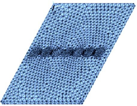
Numerical simulation is a good solution for understanding the process and helping design the FSW tools [19, 20]. A finite element simulation (FE) was carried out using APDL (ANSYS Parametric Design Language) software package to predict the residual stresses induced by the FSW technique in order to calculate the modal data of the welded plate. The brick element called SOLID70 was used to modeling the weld joint with refined meshes created near the weld area for more precise results. The element is defined by eight (08) nodes with the temperature as a single degree of freedom at each node and by the properties of the orthotropic material. The Finite Element model is illustrated in Figure 1.
The FSW modeling of flat plate is obtained according to a programming in three essential stages: thermal, structural and modal analysis as well as the input and output files associated with each of the calculation steps.
Figure 1. Finite Element Model of FSW plate
3.1 Thermal analysis
Most parameters are declared at the start of the thermal analysis program and grouped together in this first section to facilitate possible modifications. In fact, the calculation times for the resolution during the FSW welding procedure is equal to the duration of displacement of the elementary center of heat affected surfaces from one end of the plate to the other. The time of a calculation step, during heating, corresponds to the time of passage of the moving center from one element to another.
Figure 2. Schematic diagram of welding process [21]
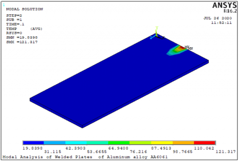
Figure 3. The temperatures at each calculated time step
The purpose of the thermal model is to calculate the transient temperature fields developed in the workpiece during friction stir welding as shown in Figure 2. The thermal analysis must be transient since the supply of a heat flux at a given point on the plate varies with time because of the movement of the heat source, is estimated by the three-dimensional nonlinear heat transfer Eq. (1).
$k\left(\frac{\partial^{2} T}{\partial x^{2}}+\frac{\partial^{2} T}{\partial y^{2}}+\frac{\partial^{2} T}{\partial z^{2}}\right)+Q_{i n t}=c \rho \frac{\partial T}{\partial t}$ (1)
where, k is the coefficient of thermal conductivity, $Q_{\text {int }}$ is the internal heat source rate, c is the mass-specific heat capacity, and ρ is the density of the materials.
The total heat input Q is given by Eq. (4) Chao et al. [21].
$Q=\frac{\pi \omega \mu F\left(r_{o}^{2}+r_{o} r_{i}+r_{i}^{2}\right)}{45\left(r_{o}+r_{i}\right)}$ (2)
where, ω is the tool rotational speed, μ is the frictional coefficient, F is the downward force, and $r_{o}$ and $r_{i}$ are the radii of the shoulder and the nib of the pin tool.
The displacement of the heat source from one node to another is carried out by a computation loop. Finally, note that the thermal solutions obtained from each loop are recorded for later use; Figure 3 shows the reading of the temperatures at each calculated time step.
3.2 Structural analysis
A structural analysis is carried out in order to obtain the residual stresses of welding. The modeling is obtained following the sequence of several analyses. This step constitutes the second phase of the simulation. In welding, the structural effect results directly from temperature gradients (thermal action).
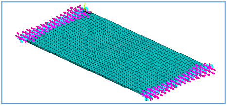
The structural analysis program uses other calculation parameters different from that defined in the thermal analysis program. The structural properties introduced in this analysis are: Poisson's ratio, Young's modulus and Density. The Element Type Change command (ETCHG) makes it possible to keep exactly the same model (geometry and mesh) created for the thermal analysis by changing only the thermal element by its structural correspondent. The boundary conditions of the FSW plate are supposed to be clamped in two sides, Figure 4.
Figure 4. The boundary conditions of FSW plate
3.3 Modal analysis
The modal analyzes performed in this calculation step use the results obtained from the thermo-structural study in order to calculate the effect of the residual stresses on the Fundamental frequencies of the FSW plate. The problem of the eigenvalue and eigenvector is solved thus used as output results.
The motion equation of the free vibration FSW plate can be obtained from Hamilton's principle, which is a generalization of the principle of displacements in the dynamics of deformable bodies:
$\delta \int_{1}^{2} L d t=\delta \int_{1}^{2}(T-\pi p) d t=0$ (3)
where, δ is the variationnelle operator, L is the Lagrange function of the FSW plate; t1 and t2 are the time limits. T is the kinetic energy; πp is the potential energy the Lagrange equations become:
$\frac{d}{d t}\left[\frac{\partial T}{\partial\left\{w_{i}^{\prime}\right\}_{e}}\right]-\frac{\partial T}{\partial\left\{w_{i}\right\}_{e}}+\frac{\partial \pi_{p}}{\partial\left\{w_{i}\right\}_{e}}=\{0\} \quad i=1,2, \ldots . n$. (4)
where, $\left\{w_{i}\right\}$ and $\left\{w_{i}^{\prime}\right\}$ are the displacement vectors and velocities of the generalized coordinates for the analysis of free vibration, the differential equations for FSW plate is written:
$\left[[K]-\omega^{2}[M]\right]\{w\}=\{0\}$ (5)
[K] and [M] are the total rigidity and total mass matrix respectively, obtained by the assembly of the elementary matrices. {w} is the global displacement vector. A non-trivial solution is therefore only possible if:
$\left|\left(K-M \omega^{2}\right)\right|=0$ (6)
Each Eigen-frequency $\omega_{i}$ corresponds to a specific mode of vibration. So for mode (i), the system of equations will be written:
$\left\{\begin{array}{c}\left(k_{11}-\omega^{2} m_{i}\right) w_{1}^{i}+k_{12} w_{2}^{i}+\ldots k_{1 n} w_{n}^{i}=0 \\ k_{21} w_{1}^{i}+\left(k_{22}-\omega^{2} m_{2}\right) w_{2}^{i}+\ldots k_{2 n} w_{n}^{i}=0 \\ \ldots \ldots . . \ldots \ldots . \ldots \ldots . . \\ k_{n 1} w_{1}^{i}+k_{n 2} w_{2}^{i}+\ldots\left(k_{n n}-\omega^{2} m_{i}^{2}\right) w_{n}=0\end{array}\right.$ (7)
We also define the spectral matrix as being:
$\omega^{2}=\left[\begin{array}{llll}\omega_{1}^{2} & & & \\ & \omega_{n}^{2} & & \\ & & . . & \\ & & & \omega_{n}^{2}\end{array}\right]$ (8)
And the modal matrix of FSW plate by:
$\phi=\left[\left\{\phi_{1}\right\}\left\{\phi_{2}\right\} \ldots\left\{\phi_{n}\right\}\right]=\left[\begin{array}{cccc}\phi_{11} & \phi_{12} & . . & \phi_{1 n} \\ \phi_{21} & \phi_{22} & . . & \phi_{2 n} \\ . . & . . & . . & . . \\ \phi_{n 1} & \phi_{n 2} & . . & \phi_{n n}\end{array}\right]$ (9)
Some commands are introduced at the beginning of the program in order to favor, on the one hand, the convergence of the calculations, especially since the behavior of the material is non-linear (temperature-dependent properties) and on the other, minimization of time Calculation time (program execution time). The total heat input Q in watts for this model is calculated through experimental and is applied as a moving heat flux. The total heat input Q of 8.15 MWatt/m2. Before representing the results of the modal analysis of the two cases (welded and virgin plates) must go through the presentation of the various results in the FSW step by the thermal study.
4.1 Thermal analyzes results
The thermal properties of the FSW plate are induced in thermal analysis, the physical characteristics of which are taken from Awang [21] in Table 2, at different stage of temperatures.
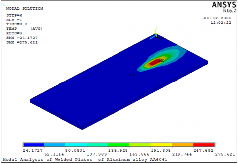
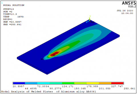
Figure 5 shows the distribution of temperatures on the upper face of the plate at different time intervals, a large part of the plate remains thermally inactive, which reflects the highly localized nature of the welding. The zone of the high-temperature gradient is then situated in the vicinity of the surface or on which the heat flow is applied ho the maximum temperature is 434.17℃.
Table 2. Physical properties for AA 6061-T6 at different temperatures
|
Temperature (℃) |
Thermal Conductivity (W/m ℃) |
Heat Cap. (J/kg℃) |
Density (Kg/m3) |
Young's Modulus E (GPa) |
Yield Strength. (MPa) |
Thermal Expansion (10-6/℃) |
|
37.80 |
162 |
945 |
2685 |
68.54 |
274.4 |
23.45 |
|
93.30 |
177 |
978 |
2685 |
66.19 |
264.6 |
24.61 |
|
148.9 |
184 |
1004 |
2667 |
63.09 |
248.2 |
25.67 |
|
204.4 |
192 |
1028 |
2657 |
59.16 |
218.6 |
26.60 |
|
260.0 |
201 |
1052 |
2657 |
53.99 |
159.7 |
27.56 |
|
315.6 |
207 |
1078 |
2630 |
47.48 |
66.2 |
28.53 |
|
371.1 |
217 |
1104 |
2630 |
40.34 |
34.5 |
29.57 |
|
426.7 |
223 |
1133 |
2602 |
31.72 |
17.9 |
30.71 |
a. Temperature after Load Step 2, time 0.1 sec
b. Temperature after Load Step 4, time 1.2 sec
c. Temperature after Load Step 6, time 3.2 sec
d. Temperature after Load Step 9, time 6.2 sec
e. Temperature after Load Step 12, time 24.17 sec
f. Temperature after Load Step 13, time 10.3 sec
g. Temperature after Load Step 16, time 25.05 sec
h. Temperature after Load Step 15, time 12.2 sec
Figure 5. The temperatures at each calculated time step
4.2 Modal analyzes results
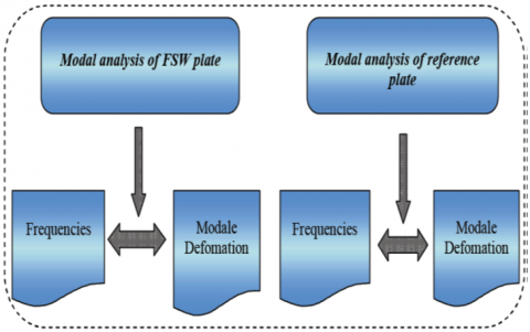
The simulation is done by following the sequence of two modal analyzes; Figure 6 shows the order in which the studies were performed.
Reference plate: it is a virgin plate with the same physical and geometrical parameters as that used for the thermal simulation. The numerical results of this model will serve as a computational reference.
FSW plate: this plate has exactly the same parameter as that used for the thermal simulation with taking into account the effect of the residual stresses in the plate.
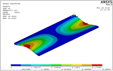
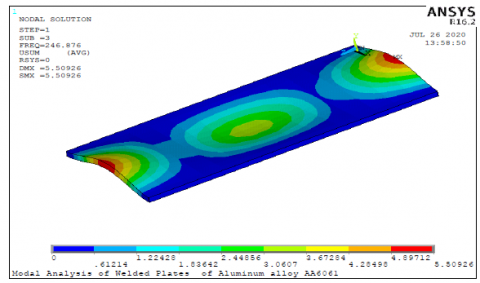
The variations of the eigenfrequencies and modal deformation in the plate are illustrated by Table 3 and Figure 7 respectively. The modal analyses carried out in this calculation step use the results obtained from the thermo-structural analysis in order to calculate the effect of the residual stresses on modal frequencies and deformations of the FSW plate.
The eigen solution is obtained with Lanczos extraction technique with an expanding method for vibration modes.
By analyzing the modal deformations obtained in Figure 7, it is possible to distinguish a variation for the deformations, consequently variations of the eigenfrequencies, of the two plates. It is noticed that the residual stresses affect significantly the response of the plate in the modal analysis; the rate of change depends on the nature of the mode (longitudinal, bending, torsion, etc.).
Figure 6. Different stages of the FSW plate analysis results
MODE 01-FSW PLATE
MODE 01- REFREENCE PLATE
MODE 02-FSW PLATE
MODE 02- REFREENCE PLATE
MODE 03-FSW PLATE
MODE 03- REFREENCE PLATE
MODE 04-FSW PLATE
MODE 04- REFREENCE PLATE
Figure 7. Variation of the modal deformation for both plate states
Table 3. Frequencies for both plate states
|
Modes |
Fundamental frequencies (Hz) |
Difference% |
|
|
Reference plate |
FSW plate |
||
|
1 |
180.82 |
217.82 |
20.46 |
|
2 |
187.21 |
223.76 |
19.52 |
|
3 |
210.05 |
246.88 |
17.53 |
|
4 |
257.70 |
320.19 |
24.25 |
The numerical values obtained with the modal analysis are listed in Table 3 which presents the percentage of variation of the fundamental frequencies for the welded plate compared to the reference plate. The impact of the residual stress on the fundamental frequencies is clearly visible where the difference between the values of the welded and reference plates represents the variation caused only by the residual stress. This difference is around 20% for all modes selected.
The main objective of this study was to examine the effect of residual stresses caused by the friction stir welding process on the modal analysis of the plate. It is evident that the effect of the heat quantity modifies the dynamic results of the plate between the "welded" and "virgin" state. This effect can be related to the increase in the plastic deformations undergone by the plate; on the other hand, it is reasonable to believe that the law of behavior used can also have an effect on the variation of the eigenfrequencies and modal deformation in the plate.
Because of these results, it would be interesting to have very different parameters in order to observe the influence of these parameters on the fundamental frequencies variation of the plate.
The analysis of the different parameters effect will allow us to better understand the factors influencing the amplitude of these variations. The parameters are as follows:
The amount of heat induced during welding;
The constitutive law of the material;
The geometric modifications undergone by the plate.
The modification of these parameters will make it possible to determine the sensitivity of the model and to make the appropriate assumptions in order to obtain a numerical result as close as possible to the real measurements.
Future work will include performing experiments with measurement of residual stresses due to the FWS process to validate and thus adjust modal parameters of dynamic simulations.
|
L |
Length of Plate, m |
|
b |
Width of plate, m |
|
h |
Thickness of plate, m |
|
E |
Young's module, GP |
|
ρ |
Mass density, Kg.m-3 |
|
T |
Temperature, ℃ |
|
t |
Time, s |
|
Q |
Total heat input, Wat.m-2 |
|
Greek symbols |
|
|
k |
Coefficient of thermal conductivity |
|
$Q_{\text {int }}$ |
Internal heat source rate |
|
ω |
The tool rotational speed |
|
μ |
Frequencies ratio |
|
c |
Mass-specific heat capacity |
|
F |
Downward force |
|
$r_{o}$ |
Radii of the shoulder |
|
$r_{i}$ |
Radii of the nib of the pin tool |
|
K |
Total rigidity matrix |
|
M |
Total mass matrix |
|
w |
The global displacement vector |
|
$\omega_{i}$ |
Specific mode of vibration |
[1] Aghdam, N.J., Hassanifard, S., Ettefagh, M.M., Nanvayesavojblaghi, A. (2014). Investigating fatigue life effects on the vibration properties in friction stir spot welding using experimental and finite element modal analysis. Strojniški Vestnik-Journal of Mechanical Engineering, 60(11): 735-741. https://doi.org/10.5545/sv-jme.2013.1324
[2] Lacki, P., Więckowski, W., Wieczorek, P. (2015). Assessment of joints using friction stir welding and refill friction stir spot welding methods. Archives of Metallurgy and Materials, 60(3): 2297-2306. https://doi.org/10.1515/amm-2015-0377
[3] Pamuk, M.T., Savaş, A., Seçgin, Ö., Arda, E. (2018). Numerical simulation of transient heat transfer in friction-stir welding. International Journal of Heat and Technology, 36(1), 26-30. https://doi.org/10.18280/ijht.360104
[4] Simar, A., Bréchet, Y., De Meester, B., Denquin, A., Gallais, C., Pardoen, T. (2012). Integrated modeling of friction stir welding of 6xxx series Al alloys: process, microstructure and properties. Progress in Materials Science, 57(1): 95-183. https://doi.org/10.1016/j.pmatsci.2011.05.003
[5] Jabbari, M. (2013). Effect of the preheating temperature on process time in friction stir welding of Al 6061-T6. Journal of Engineering, Vol. 2013. https://doi.org/10.1155/2013/580805
[6] Nandan, R., Roy, G.G., Debroy, T. (2006). Numerical simulation of three-dimensional heat transfer and plastic flow during friction stir welding. Metallurgical and Materials Transactions A, 37(4): 1247-1259. https://doi.org/10.1007/s11661-006-1076-9
[7] Chao, Y.J., Qi, X., Tang, W. (2003). Heat transfer in friction stir welding-experimental and numerical studies. Journal of Manufacturing Science and Engineering, 125(1): 138-145. https://doi.org/10.1115/1.1537741
[8] Vishwanath, M.M., Lakshamanaswamy, N., Ramesh, G.K. (2019). Numerical simulation of heat transfer behavior of dissimilar AA5052-AA6061 plates in fiction stir welding: an experimental validation. Strojnícky časopis-Journal of Mechanical Engineering, 69(1): 131-142. https://doi.org/10.2478/scjme-2019-0011
[9] Vilaça, P., Quintino, L., dos Santos, J.F. (2005). iSTIR-analytical thermal model for friction stir welding. Journal of Materials Processing Technology, 169(3): 452-465. https://doi.org/10.1016/j.jmatprotec.2004.12.016
[10] Ji, S.D., Shi, Q.Y., Zhang, L.G., Zou, A.L., Gao, S.S., Zan, L.V. (2012). Numerical simulation of material flow behavior of friction stir welding influenced by rotational tool geometry. Computational Materials Science, 63: 218-226. https://doi.org/10.1016/j.commatsci.2012.06.001
[11] Xue, C., Ren, X., Zhang, Q. (2013). Heat production simulation and heat-force couple analysis of FSW pin. Materials Science, 33(2), 85-91.
[12] Zhao, Y.H., Lin, S.B., Wu, L., Qu, F.X. (2005). The influence of pin geometry on bonding and mechanical properties in friction stir weld 2014 Al alloy. Materials Letters, 59(23): 2948-2952. https://doi.org/10.1016/j.matlet.2005.04.048
[13] Boz, M., Kurt, A. (2004). The influence of stirrer geometry on bonding and mechanical properties in friction stir welding process. Materials & Design, 25(4): 343-347. https://doi.org/10.1016/j.matdes.2003.11.005
[14] Zhu, X.K., Chao, Y.J. (2004). Numerical simulation of transient temperature and residual stresses in friction stir welding of 304L stainless steel. Journal of Materials Processing Technology, 146(2): 263-272. https://doi.org/10.1016/j.jmatprotec.2003.10.025
[15] Ameen, H.A., Hassan, K.S., Salah, M.M. (2011). Influence of the butt joint design of TIG welding on the thermal stresses. Engineering and Technology Journal, 29(14): 2841-2858.
[16] Abdul-Sattar, M., Tolephih, M.H., Jweeg, M.J. (2012). Theoretical and experimental investigation of transient temperature distribution in friction stir welding of AA 7020-T53. Journal of Engineering, 18(6): 693-709.
[17] Li, H., Liu, D. (2014). Simplified thermo-mechanical modeling of friction stir welding with a sequential FE method. International Journal of Modeling and Optimization, 4(5): 410. https://doi.org/10.7763/IJMO.2014.V4.409
[18] Zahari, S.N., Sani, M.S.M., Husain, N.A., Ishak, M., Zaman, I. (2016). Dynamic analysis of friction stir welding joints in dissimilar material plate structure. Jurnal Teknologi, 78(6-9). https://doi.org/10.11113/jt.v78.9148
[19] Liu, H.J., Feng, J.C., Fujii, H., Nogi, K. (2005). Wear characteristics of a WC-Co tool in friction stir welding of AC4A+ 30 vol% SiCp composite. International Journal of Machine Tools and Manufacture, 45(14): 1635-1639. https://doi.org/10.1016/j.ijmachtools.2004.11.026
[20] Lin, S.B., Zhao, Y.H., He, Z.Q., Wu, L. (2011). Modeling of friction stir welding process for tools design. Frontiers of Materials Science, 5(2): 236-245. https://doi.org/10.1007/s11706-011-0128-2
[21] Awang, M. (2007). Simulation of friction stir spot welding (FSSW) process: study of friction phenomena. West Virginia University.