Soumia Ourrad* | Youcef Houmadi | AbdelKader Ziadi | Sidi Mohammed Aissa Mamoune | Abdelkader Lousdad
OPEN ACCESS
This study investigated the effect of hydrogen on reduction in area in relation to the storage time of a high carbon steel wire for C-Mn pre-stressed concrete in the context on hydrogen embrittlement of steel. The Monte Carlo Simulation method was employed for the probabilistic analysis. The concentration of hydrogen "C∞", the effective diffusion coefficient "De" these parameters were considered as random fields. The probabilistic response considered in the analysis was the reduction in area "Z". Numerical simulations that make use of second Fick’s law were used for the computation of this response. A parametric study was undertaken to investigate the effect of the input and the statistical parameters of the random variables on the probability distribution functions of the response. Also, this study contributes to bring more elements of comprehension on the spatial and temporal variability of the input and output parameters.
ductility, hydrogen embrittlement, spatial variability, stochastic method, Karhunen-Loève
Steel wire for pre-stressed concrete, is a twisted steel cable composed of several high strength steel wires and is stress-relieved (stabilized) for pre-stressed concrete. The safety and durability of these materials are seriously compromised by the degradation of materials in the presence of hydrogen. Hydrogen embrittlement is a common phenomenon that degrades metals [1-7]. Over the last hundred years, many failures have been identified in metals that can be attributed to the damage caused by hydrogen. Avoiding the presence of hydrogen is extremely difficult in certain situations: hydrogen is linked to corrosion processes, produced in humid and acidic environments [8-9]. Pre-stressed concrete steel wire is made of hot-rolled, high-carbon steel that must be drawn- to the required final diameter. It is well-known that, during this operation, hydrogen produces a dangerous effect on steel ductility [10-11].
The effect of the uncertainties of the steel wire road parameters on the reduction of area "Z" has never been studied in the literature. The analysis approach based on the probabilistic method is the most reliable way to solve uncertainty problems. The latter has attracted a lot of interest from researchers recently. As reliability concepts are better understood and more software developed, reliability-based applications move from simple, hypothetical examples using fictitious data to more complex, practical, and realistic engineering problems [10].
The present work aims to predict an optimum time for hydrogen desorption using a spatial variability approach. This approach takes into account the spatial variability of the different parameters such as hydrogen concentration (Chyd) and effective diffusion (De) appearing in simple model.
The probabilistic analysis approaches the problems in a completely different way by using Monte Carlo Simulation method (MCS), by postulating the random nature of input parameters which is concentration and diffusion to involve in the phenomena studied and in the behavior models used to describe these phenomena. This method is used to compute the Probability Distribution Function (PDF) of the response or the failure probability. It is a robust method that gives reliable results with low errors.
2.1 Deterministic analysis
The commercial grade steel used in this study was produced as a hot-rolled and controlled-cooled wire rod with 11mm diameter. Its chemical composition (in weight percent) is mentioned in Table 1.
The modeling of hydrogen desorption is established that the passage of hydrogen through steel is hindered by lattice imperfections which tend to attract and bind it, thus rendering it immobile at temperatures where it should normally be able to diffuse readily [12].
Table 1. Chemical composition of steel [11]
|
Elements |
C |
Mn |
P |
S |
Si |
Al |
N |
|
Rate % |
0.82 |
0.77 |
0.015 |
0.004 |
0.12 |
0.0021 |
0.0040 |
The origin of the lattice diffusion of hydrogen in a metal is the hydrogen concentration gradient between the surface and the inside of the metal created by absorption of hydrogen. The reticular diffusion of hydrogen consists of a series of jumps from one interstitial site to the next one. These jumps require activation energy for crossing the energy barrier between two sites. The first and second Fick's laws conventionally describe the lattice diffusion of hydrogen in the absence of any other driving force, the stress gradients, temperature or existence of an electric field which can also be the cause of hydrogen diffusion [13-14].
2.2 Mathematic model
Fick’s first law describes the change in concentration over time as the following:
$J=-D \nabla \phi$ (1)
where, J is the diffusive flux of hydrogen atoms in $\mathrm{mol} / \mathrm{m}^{2} \mathrm{s}$ is the diffusion coefficient in $\mathrm{m}^{2} / \mathrm{s}, \nabla$ is the gradient operator, for many material problems it is not the flux that is
as important as the concentration at any given time [15].
The second Fick's law [15] gives a relation which describes the variation of the concentration gradient according to time and is expressed by Equation 2:
$\frac{\partial C_{h y d}}{\partial t}=-D \nabla^{2} C_{h y d}$ (2)
where, Chyd is the concentration gradient in $\mathrm{mol} / \mathrm{m}^{3}$.
By reducing it in cylindrical coordinates form, we obtain:
$\frac{\partial C_{hyd}}{\partial t}=D \frac{\partial^{2} C_{\operatorname{hyd}}}{\partial r^{2}}$ (3)
By considering the following initial and boundary conditions:
$C(r, 0)=C_{0}$ for $0 \leq r \leq R$ and $t=0$ (4)
$\frac{\partial C}{\partial r}=0 \quad$ for $\quad r=0$ and $\quad t>0$ (5)
$C(R, t)=\operatorname{Coo}$ for $r=R$ and $t>0$ (6)
where, r is radius and R is radius of wire road
The exact solution of Eq. (2), considering conditions calculated by Eqns. (4)-(6), is as follows [15]:
$\frac{c(r, t)-c_{0}}{c_{\infty}-c_{0}}=1-\frac{2}{R} \sum_{n=1}^{\infty} \frac{\exp \left(-D \alpha_{n}^{2} t\right) J_{0}\left(\alpha_{n}^{2} r\right)}{\alpha_{n}^{2} J_{1}\left(\alpha_{n}^{2} R\right)}$ (7)
$\alpha_{n}=\frac{(4 n-1) \pi}{4 R}=\frac{(4 n-1) \pi}{2 d}$ (8)
Provided the $\alpha_{\mathrm{n}}$ are positive roots of Bessel function and d is the diameter.
Using only the first term of this series and considering an effective diffusion coefficient De for trap-controlled diffusion and $C_{t}$ mean hydrogen concentration at time $t$ and $C_{0}$ is concentration at time $t=0$ lead to the following equation:
$\frac{C_{t}-C_{\infty}}{C_{0}-C_{\infty}}=\frac{64}{9 \pi^{2}} \exp \left[-\left(\frac{3 \pi}{2 d}\right) D_{e} \mathrm{t}\right]$ (9)
$C_{t}=C_{\infty}+0.72\left(C_{0}-C_{\infty}\right) \exp \left(\frac{-22.2 D_{e} t}{\mathrm{d}^{2}}\right)$ (10)
By assuming a linear relation between “Z” where is the reduction in area and concentration:
$Z=Z_{0}+E\left(C_{0}-C_{t}\right)$ (11)
By replacing Eq. (11) in Eq. (10) we obtain:
$Z=Z_{0}+E\left(C_{0}-C_{\infty}\right)\left[\left(1-0.72 \exp \left(\frac{-22.2 D e t}{\mathrm{d}^{2}}\right)\right)\right]$ (12)
2.3 Probabilistic analysis
Direct Simulation Method of Monte Carlo consists of conducting a large number of simulation $N_{s}$ (prints) of the random variables of the studied problem for each simulation. The state function is calculated and there are simulations leading to failure of the $N_{s f}$ structure. The failure probability $P_{f}$ is then estimated by the ratio between the numbers of simulations $N_{s}$ leading to failure and the total number of $N_{s}$ prints:
$P_{f}=\frac{N_{s f}}{N_{s}}$ (13)
where, N is the total number of simulations. This failure probability estimator can also be written as follows [16-17]:
$P_{f}=\frac{1}{N_{S}} \sum_{1}^{N} I[G(X)]$ (14)
where, I (G(x)) is the domain of the lack of safety (failure), it is equal to 1 in unsafe areas and it is equal to 0 in the safe zone.
$I[G(x)]=\left\{\begin{array}{l}{1 \text { if } G(x) \leq 0} \\ {0 \text { if } G(x)\rangle 0}\end{array}\right\}$ (15)
In this work a probabilistic analysis is performed on the reduction in area of a heterogeneous steel rod used in pre-stressed concrete whose properties are spatially variable by determining the mean values of the concentration and diffusion coefficient and coefficient of variation (COV). In this study the random fields of these properties were discretized into a finite number of random variables using the Karhunen-Loeve expansion (KL). The illustrative values used for the statistical moments of the different random variables are those commonly encountered in practice [11]. These are given in Tables 2 and 3.
Table 2. Initial values of hydrogen content, C0, tensile strength and reduction in area, Z, of the studied steel
|
Parameters |
Co (ppm) |
Z (%) |
|
Measured value |
1.85 |
20±2 |
|
Specified value (state function G) |
/ |
≥30 |
Table 3. Input model data
|
Parameters |
Mean |
Coefficient of variation (COV) |
|
$\mathbf{C}_{\infty}$ (ppm) |
0.56 |
0.06 |
|
De (mm2/s) |
0.08 |
0.13 |
The accuracy of the estimated failure probability can be measured by calculating its coefficient of variation as follows:
$\partial P_{f}=\sqrt{\frac{1-P_{f}}{P_{f} N_{s}}}$ (16)
In the literature, we can find several methods of discretization proposed by the researchers, which consist of breaking down the initial fields into optimal complete deterministic functions [18-19]. To do this, the discretization of a section involves a subdivision of the sample structure into small pieces of random field in the direction of the x-axis and the y-axis, as shown in Figure 1. But, the discretization with more elements provides more accurate results but also requires more computing time.
The transition from the representation of the continuous random field to a limited number of random variables is necessary to introduce the uncertainty of the properties of the materials into a computation model. To do this, we must choose a discretization method. In this study, the Karhunen-Loève expansion method (K-L) was adopted for the sample discretization.
Figure 1. Dimensional discretization model
where, n is the number of elements along the x-axis which is equal to 10 elements with a pitch n equal to 40 mm and m is the number of elements following the y-axis which is equal to 10 elements with a pitch m equal to 9.5 mm .The random field was discretized using the expansion of Karhnuen-Loeve (KL). According to this method, it provides a good approximation of the random field H ($\mathrm{X}, \theta$) [20-23].
$H(X, \theta)=\mu+\sum_{i=1}^{\infty} H_{i}(X) \xi_{i}(\theta)$ (17)
To introduce uncertainty of material properties in a computational model it is necessary to move from the representation of continuous random field H (X) to a limited number of random variables. To do this one must choose a discretization method. These approaches are various and can be divided into three categories: point method, the discretization average method and series expansion method. In this paper we used the expansion Karhunen-Loève (KL) which belongs to the series expansion method. The KL expansion provides a characterization of the second-moment of a random process in terms of deterministic orthogonal functions and non-correlated random variables as a result [24].
The approximate random field is defined by truncating the ordered series by taking the value M instead of $\infty$:
$H(X, \theta) \rightarrow H(H, \theta)=\mu+\sum_{i=1}^{\infty} H_{i}(X) \xi_{i}(\theta)$ (18)
$H_{i}(X)=\sqrt{\lambda_{i}} \varphi_{i}(x)$ (19)
With:
$\xi_{i}(\theta):$ Uncorrelated Random variable, $\mu=0$ et $\sigma^{2}=1$
θ: indicates the random nature of the corresponding amount
X: spatial coordinates in the physical space
Eigen vectors and eigen values of autocorrelation function.
In our case we took M equal to 200; the choice of the number M of terms depends on the desired accuracy of the problem being treated
In this study the different values of the distance of horizontal and vertical autocorrelation were studied and analyzed.
The limit state function used to calculate the failure probability is defined as follows:
$G=Z_{\mathrm{lim}}-Z$ (20)
where, $Z_{\lim }$ = 30 %.
It should be emphasized here that this study makes use Monte Carlo Simulation (MCS) methodology to compute the Probability Distribution Function (PDF) of the system response or the failure probability.
3.1 Influence of autocorrelation distances
A parametric study was performed to determine the effect of autocorrelation distances Lx and Ly on failure probability.
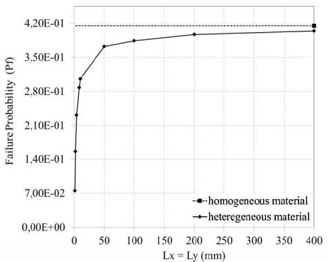
Figure 2 shows the effect of the autocorrelation distance on the failure probability. For the case of isotropic random field (Lx = Ly). This figure also shows the failure probability corresponding to homogeneous material. The failure probability was calculated on the supposition that the material is homogeneous and has the same average values of the random variables along the sample.
Figure 2. Effect of autocorrelation distances (Lx and Ly) on failure probability in the case of an isotropic random field
In this case, the failure probability has been calculated and has the same average values as the random variables.
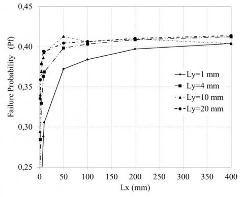
In order to study the effect of the anisotropy of random field, the failure probability it presented as a function of vertical and horizontal autocorrelation distance in Figure 3 and 4, respectively.
Figure 3. Effect of horizontal autocorrelation distance on the failure probability for different Lx values
The increase in the failure probability due to the increase of the autocorrelation distance can be explained as follows: when the autocorrelation distance is very large the material tends to be homogeneous. In this case, the reduction in area was judged too close to that obtained during the study of homogeneous material. For smaller autocorrelation distances a heterogeneity of material is obtained which results in a variability of the random variables which has a significant influence on the reduction in area. In this case the reduction in area is important by some large sections of the random variables and is low in other sections with low value of these variables.
Figure 4. Effect of vertical autocorrelation distance on the failure probability
The increase in the failure probability due to the increase of the autocorrelation distance can be explained as follows: when the autocorrelation distance is very large the material tends to be homogeneous. In this case, the reduction in area was judged too close to that obtained during the study of homogeneous material. For smaller autocorrelation distances a heterogeneity of material is obtained which results in a variability of the random variables which has a significant influence on the reduction in area. In this case the reduction in area is important by some large sections of the random variables and is low in other sections with low value of these variables.
The interest of this study is to define the order of the autocorrelation distances, so note that the configurations used in this study correspond to the autocorrelation distances equal to 50 for the x-axis and 20 for y-axis. It will likewise be taken for probabilistic calculations carried out for the present study.
3.2 Study of the spatial and temporal variability of autocorrelation distances
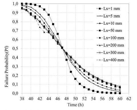
In this section the failure probability is analyzed and interpreted for different scenarios. For small autocorrelation distances (Lx < 25 mm & Ly < 2 mm), it should be noted that Pf decreases more slowly before the inflection point and reverses immediately after the inflection point. This results in a heterogeneity of the material which causes the hydrogen release more easily. However for the other Lx and Ly we notice that the curves of Pf decrease faster before the point of inflection and decrease more slowly just after this point knowing that the plots are almost superimposed which explains that the material is less heterogeneous (Figure 5).
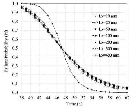
For longer autocorrelations distances (Lx>25mm & Ly>2mm) it should be noted that failure probability decreases relatively fast and keeps the same rate for all levels of Lx and the maximum value for Ly is equal to 8mm (Figure 6). The hypothesis that the material tends towards the homogeneity of the material which slows down the escape of hydrogen from the sample.
This result only confirms the previous result concerning the homogeneity of the material concerning the large values of autocorrelation distances but it provides more understanding for time evolution because it gives us the look of follow analysis a study according to time and according to random variables.
Figure 5. Time evolution of the failure probability for different positions of Lx
Figure 6. Time evolution of failure probability for different positions of Ly
3.3 Computational time optimization
For the probabilistic analysis, the Monte Carlo Simulation (MCS) methodology it generally used to compute either the Probability Density Function of the system response or the failure probability Pf.
Inspire of being a rigorous and robust methodology the MCS requires a great number of trials for the deterministic model (about one million samples for a failure probability of 1.E-5) [25].
Using equation 29, the coefficient of variation of failure probability COV(Pf) was calculated and shown in Figure 7. It has been found that it decreases with the increase in the number of simulations. It reaches to a value of coefficient of variation equal to 15% when the number of simulations Ns is equal to 10000 simulations (to Pf=10-3). For a number of simulation runs equal to Ns=100 in a low computation time but the results are unreliable ie COV(Pf)>20% for Pf>10-3. Thus it is more reasonable to limit the number of simulation runs to 10000.
Figure 7. Optimization of computational time by the number of simulations according to time
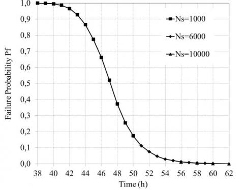
In order to save more time, it is necessary to associate each hydrogen degassing time interval with a specific number of simulations, as shown in Table 4, in order to obtain the typical profile shown in Figure 8. However, the Pf decreases with increasing time which increases the number of simulations automatically in order to have reliable Pf.
Table 4. Adaptation time calculated on function of simulation number
|
Time interval |
Simulation Number |
|
[20-50] |
1000 |
|
[51-54] |
6000 |
|
[56-62] |
10000 |
Figure 8. Time evolution of the Pf according to the number of simulation
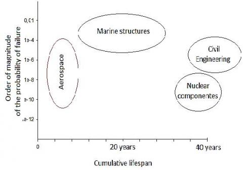
Since the steel wire used for pre-stressed concrete, it is more reasonable to compare it with the failure probability of civil engineering level according to level curve of probabilities estimated in different industrial branches (Figure 9).
Figure 9. Level of probabilities estimated in different industrial branches [26]
3.4 Parametric study
In the following subsection a sensitive analysis based on parametric study of random variables is made in order to provide the contribution of each of these variables namely the effective diffusion coefficient (De) and the concentration at a given time (C∞) on the variability of the system response the reduction in area (Z).
A study of the failure probability as function of storage time of the steel is carried out. This time allows the desorption of the hydrogen from the samples which is used in pre-stressed concrete according to our case. The limit state criteria are the reduction in area criteria which must be greater or equal to 30 %.
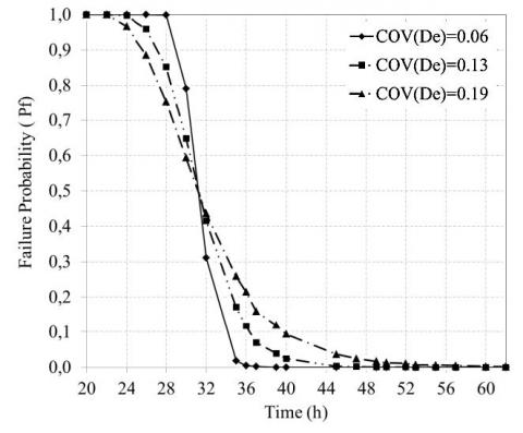
The effect of diffusion coefficient on failure probability is shown in Figure 10 and 11. Figure 10 shows that for COV(De)=0.06 failure probability is maximum up to 28hours unlike COV (De) =0.19 that failure probability begins to decline to 21 hours and COV (De) = 0.13 for which failure probability begins to decrease to 24hours. Also between 29 and 34 hours there is a convergence at the inflection point in failure probability of different diffusion coefficients (De), 32 h after failure probability for both COV (De) of 0.19 and 0.13 is reversed then decreases more slowly.
Figure 10. Time evolution of failure probability for different COV (De)
For a low values of COV (De) =0.06, the diffusion values converge to this effect. The Pf decreases rapidly in contrast to the important COV (De) where the diffusion values diverge which is the reason why the Pf decreases more slowly. N For great values of COV (De) =0.19, the large diffusion values precipitated the hydrogen release which accelerated the decrease of Pf before the point of inflection. However the low values of the diffusion slowed the escape of the hydrogen which reduces the decrease of failure probability after the inflection point. It can be concluded that the variability of the diffusion coefficient such as random fields has a significant impact on failure probability. Therefore the importance of this study which takes into account the spatial variability of material.
Figure 11. Focusing on the time interval of 35-62 hours in case of Pf according to time
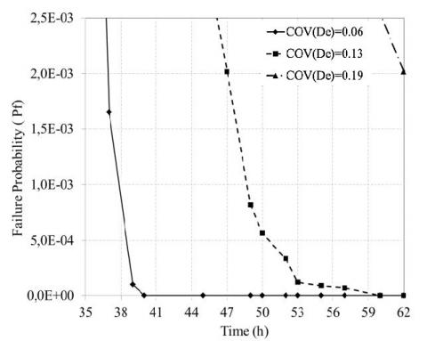
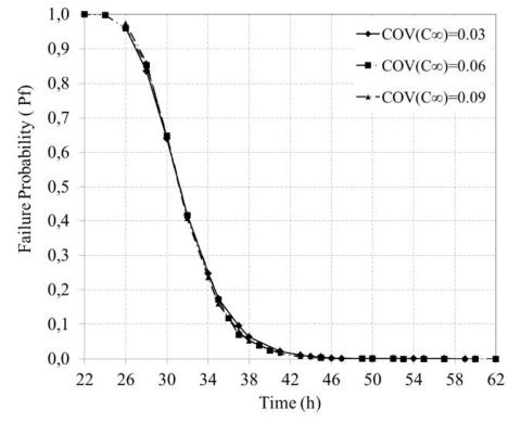
The results in Figure 12 show that the decrease in the failure probability for the three COV (C∞) is starting from 24h and then failure probability tends to zero at 43h.
Figure 12. Time evolution of failure probability for different COV (C∞)
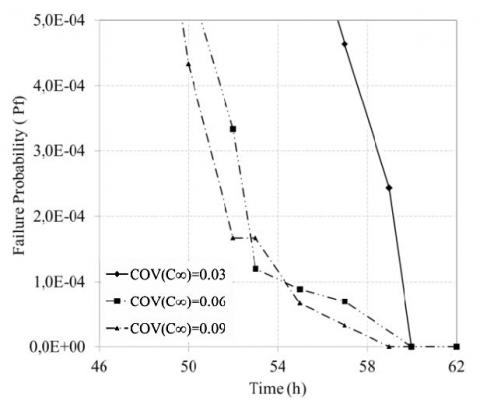
In the case where the Pf was estimated on a normal scale, i.e. 0<Pf<1, the curves of the COV(C∞) were practically coincident but were reduced to a more accurate scale. The Pf value is between 0 and 5.0E-04, in our case Pf is equal to 5.0E-04 and it is between 10-7 and 10-3 with reference to Maurice LEMAIR curve. It is to highlight that the Pf is always included in the intervals prior to Level curves as shown in Figure 9.
It is noted that there is a distinct difference so that the greater value of COV (C∞) =0.09 decreases more rapidly and reaches the probability of zero failure after 59 hours against the lower value of the COV (C∞) = 0.03 which reaches the probability of zero failure after 60 hours (Figure 13).
Figure 13. Focusing on the time interval of [48-60] hours in case of Pf according to time
The COV of reference which is equal to 0.06 after 62 hours reaches the zero failure probability. It can be concluded that the concentration parameter has a minor impact on the phenomenon of hydrogen desorption compared to the diffusion parameter.
This Paper aims at presenting a probabilistic analysis at serviceability limit state of reduction in area of hydrogen desorption phenomenon in the steel rod for pre-stressed concrete C-Mn with a spatially varying effective diffusion coefficient (De) and concentration (C∞) using Monte Carlo simulation method. The deterministic model was based on the first according second Fick’s laws conventionally describe the lattice diffusion of hydrogen implemented in MATLAB software. The main conclusions of the present paper can be summarized as follows:
(1) A parametric study has shown that the variability of reduction in area Z was mainly induced by effective diffusion coefficient (De). Concentration parameter (C∞) has a minor effect in response variability and this parameter can be considered as deterministic. The strategy of detecting the most influential parameters that significantly reduces the computation time of the probabilistic analysis by software simulation. One of the main practical obstacles to these methods is the very high computation time of numerical models combined with the large number of simulations to these models necessary for the application of probabilistic methods hence the value of the computational time optimization study which has reduced the time and computational cost for the present study and for the future perspectives. It has also the advantage of reducing the cost of experimental investigation of new similar projects because the less-influential parameters do not need a thorough experimental investigation on their variability’s
(2) The fields (De and C∞) were discretized into a finite number of random variables using the Karhunen-Loève expansion. Therefore the input uncertain parameters that have a significant impact in the variability of this response are the effective diffusion (De) should be thoroughly investigated in practice. In fact that in a reduced cross section where the autocorrelation distances are much smaller we note that a heterogeneity of material which results by the variability of diffusion coefficient. The most likely explanation is that in a great heterogeneity in area there are more microstructural defects at room temperature that facilitate diffusion of hydrogen. In contrast to a larger section the material tends to homogeneity involving less defects leading to the slowing down of hydrogen diffusion.
(3) The standard deviation of the system response increases with the increase of the Coefficient of Variation of inputs random fields. Concerning the mean value it remains quite constant in diffusion parameter.
(4) Finally, the validation of our obtained results is made by comparing them with those obtained by Carneiro’s [11]. It should be noted that the optimal storage time deduced from the deterministic approach by Carneiro is greater than that its around 98hours for storage time to reach a required reduction in area. For probabilistic approach and especially for a failure probability equal to 10-3 which means a great precision and the required reduction in area is around 30 % is reached at 62h for storage time. As a result we obtain a gain equal to 36hours of storage time and this duration ensures obtaining the ductility required for the use of this material. This will guarantee a saving of storage time and consequently an economic gain for large quantities of this steel. However, it is desirable to involve probabilistic methods in feasibility studies for more reliable and economic decision-making. Also these approaches contribute in the decrease of the cost of the future experimental studies.
Recommendations for future studies are needed to reduce the calculation time and the coefficient of variation, it is recommended to use in similar studies the subset simulation method as an alternative to the Monte Carlo Simulation (MCS) method. Also the method of descritization EOLE can be used of interest to increase the precision of the results.
The project presented in this article is supported by the Ministry of high Education and scientific research.
|
J |
Diffusive flux, mol/m2 s |
|
D |
Diffusion coefficient , m2 /s |
|
Chyd |
Concentration,mol/m3 |
|
t |
Time, s |
|
r |
Radius, m |
|
R |
Radius of wire road, m |
|
d |
Diameter, m |
|
Z |
Reduction in area at fracture, % |
|
E |
Constant of Eq. 11 |
|
Greek symbols |
|
|
$\nabla$ |
Gradient operator |
|
$\alpha_{\mathrm{n}}$ |
Positive roots of Bessel function |
|
Subscripts |
|
|
$\infty$ |
At time t =∞ |
|
0 |
At time t=0 |
|
e |
Effective |
|
t |
At time t |
[1] Bernstein, I. (1970). The role of hydrogen in the embrittlement of iron and steel. Materials Science and Engineering, 6(1): 1-19. https://doi.org/10.1016/0025-5416(70)90073-X
[2] Delafosse, D., Magnin, T. (2001). Hydrogen induced plasticity in stress corrosion cracking of engineering systems. Engineering Fracture Mechanics, 68(6): 693-729. http://dx.doi.org/10.1016/S0013-7944(00)00121-1
[3] Gangloff, R.P., Somerday, B.P. (2012). Gaseous hydrogen embrittlement of materials in energy technologies: Mechanisms, modelling and future developments (Vol. 2), Elsevier. https://doi.org/10.1533/9780857095374
[4] Hirth, J. (1980). Effects of hydrogen on the properties of iron and steel. Metallurgical Transactions A, 11(6): 861-890. https://doi.org/10.1007/BF02654700
[5] Lynch, S.P. (2007). Progress towards understanding mechanisms of hydrogen embrittlement and stress corrosion cracking. NACE Corrosion conference, Nashville, USA.
[6] Oriani, R.A. (1970). The diffusion and trapping of hydrogen in steel. Acta Metallurgica, 18(1): 147-157. http://dx.doi.org/10.1016/0001-6160(70)90078-7
[7] Kittel, J., Smanio, V., Fregonese, M., Garnier, L., Lefebvre, X. (2010). Hydrogen induced cracking (HIC) testing of low alloy steel in sour environment: Impact of time of exposure on the extent of damage. Corrosion Science, 52(4): 1386-1392. http://dx.doi.org/10.1016/j.corsci.2009.11.044
[8] Shipilov, S.A., Le May, I. (2006). Structural integrity of aging buried pipelines having cathodic protection. Eng Failure Analysis, 13(7): 1159-1176. http://dx.doi.org/10.1016/j.engfailanal.2005.07.008
[9] Zhong, Z.Q., Tian, Z.L., Yang, C., Lin, S.P. (2015). Failure analysis of vessel propeller bolts under fastening stress and cathode protection environment. Engineering Failure Analysis, 57: 129-136. http://dx.doi.org/10.1016/j.engfailanal.2015.07.013
[10] Cherifi, W., Houmadi, Y., Benali O. (2019). Probabilistic analysis for estimation of the initiation time of corrosion. Mathematical Modelling in Civil Engineering, 15(2): 1-13. https://doi.org/10.2478/mmce-2019-0004
[11] Carneiro Filho, C.J., Mansur, M.B., Modenesi P.J., Gonzalez, B.M. (2010). The effect of hydrogen release at room temperature on the ductility of steel wire rods for pre-stressed concrete. Materials Science and Engineering: A, 527(18-19): 4947-4952. https://doi.org/10.1016/j.msea.2010.04.042
[12] Moriconi, C. (2012). Modélisation de la propagation de fissure de fatigue assistée par l'hydrogène gazeux dans les matériaux métalliques. Thèse de doctorat ENSMA-Poitiers, France.
[13] Smanio-Renaud, V. (2008). Etude des mécanismes de Fragilisation Par l'Hydrogène des aciers non alliés en milieu H2S humide: Contribution de l'émission acoustique. PhD Thesis. 'INSA Lyon, France.
[14] Crank, J. (1975). The mathematique of diffusion by BRUNEL second edition university combridge.
[15] Shewmon, P.G. (1989). Diffusion in Solids, second ed., The Minerals, Metals and Materials Society, Warrendale, PA, USA.
[16] Brandes; E.A., Brook, G.B. (1992). Smithells Metals Reference Book, Elsevier Science & Technology Books, Butterworth-Heinemann, Oxford.
[17] Houmadi, Y., Ahmed, A., Soubra, A.H. (2012). Probabilistic analysis of a one-dimensional soil consolidation problem. Georisk: Assessment and Management of Risk for Engineered Systems and Geohazards, 6(1): 36-49. https://doi.org/10.1080/17499518.2011.590090
[18] Houmadi, Y. (2011). Prise en compte de la variabilité spatiale des paramètres géotechniques thèse de doctorat. Risk Assesment and Management Laboratory "RISAM" – Tlemcen University, Algeria.
[19] Vanmarcke, E.H., Grigoriu, M. (1983). Stochastic finite element analysis of simple beams. Journal of Eng Mechanics, https://doi.org/10.1061/(ASCE)0733-9399(1983)109:5(1203)
[20] Spanos, P.D., Ghanem, R. (1989). Stochastic finite element expansion for random media. Journal of Engineering Mechanics, 115(5): 1035-1053. https://doi.org/10.1061/(ASCE)0733-9399(1989)115:5(1035)
[21] Sudret, B., Berveiller, M. (2008). Stochastic finite element methods in geotechnical engineering. In: Reliability-Based design in Geotechnical Engineering: Computations and applications, Taylor & Francis (Eds.), New York,USA, pp. 260-297.
[22] Ourrad, S., Houmadi, Y., Belzunce, F.J., Ziadi, A. (2016). Numerical analysis of Hydrogen embrittlement of high strength steels using Monte Carlo method. 7th African Conference of Nondestructive Testing Acdnt.
[23] Spanos, P.D., Ghanem, R. (1989). Stochastic finite element expansion for random media. Journal of Engineering Mechanics, 115(5): 1035-1053. https://doi.org/10.1061/(ASCE)0733-9399(1989)115:5(1035)
[24] Spanos, P.D., Ghanem, R. (1991). Spectral stochastic finite element formulation for reliability analysis. Journal of Engineering Mechanics, 117(10): 2351-2372. https://doi.org/10.1061/(ASCE)0733-9399(1991)117:10(2351)
[25] Ahmed, A. (2013). Probabilistic analysis of shallow foundations: Simplified and advanced approaches for the probabilistic analysis of shallow foundations. LAP Lambert Academic Publishing.
[26] Lemaire, M., Chateauneuf, A., Mitteau, J.C. (2009). Structural reliability. ISTE Ltd. edition. ISBN-13: 978-1848210820