
Hanani Farhah Harun
© 2026 The author. This article is published by IIETA and is licensed under the CC BY 4.0 license (http://creativecommons.org/licenses/by/4.0/).
OPEN ACCESS
This study investigates a semiparametric option-pricing framework, the Extended Generalised Leland (EGL) model, which combines transaction-cost-adjusted replication with model-free variance information. Unlike fully parametric models, such as Black–Scholes–Merton (BSM), which rely on restrictive assumptions, and purely nonparametric approaches, which often suffer from numerical instability and infeasibility, the EGL framework balances structural realism with flexibility. The models were evaluated in an advanced Quasi-Monte Carlo (QMC) simulation environment, in which asset prices were generated by a stochastic volatility jump–diffusion process. Variance reduction was achieved through Sobol low-discrepancy sequences (a deterministic alternative to pseudo-random sampling) and antithetic variates. Across 100,000 simulated paths and wide parameter ranges, the EGL (Advanced) model achieved the lowest Root Mean Squared Error (RMSE = 0.0561) and Mean Absolute Relative Percentage Error (MARPE = 4.31%) among all benchmarks. The benchmarks comprised BSM, Heston, the model-free Bakshi–Kapadia–Madan (MFBKM) method, and a calibrated artificial neural network. Statistical significance was confirmed using analysis of variance (ANOVA) with post-hoc Tukey tests. The analysis is simulation-based and does not include real-market calibration. Nevertheless, the results suggest that the EGL framework provides a robust and computationally viable alternative for derivative valuation. Future research should focus on empirical validation and extensions to multi-asset derivatives.
semiparametric option pricing, stochastic volatility jump–diffusion, Quasi-Monte Carlo simulation
1.1 Limitations of traditional parametric models
The Black–Scholes–Merton (BSM) model remains a cornerstone of option pricing theory [1, 2]. However, its restrictive assumptions (constant volatility, frictionless markets, and continuous hedging) have been repeatedly challenged, particularly during periods of market stress [3, 4]. Empirical anomalies such as volatility smiles and smirks reveal systematic pricing biases that cannot be reconciled within the BSM framework. Subsequent parametric extensions, including stochastic volatility and jump–diffusion models, improve realism but remain sensitive to model misspecification and parameter calibration [5, 6]. More generally, parametric models often rely on stringent and unrealistic assumptions about market dynamics, which can lead to substantial underpricing of options [7, 8]. Janková [9] highlighted the problem posed by the constant-volatility assumption and noted that such constraints frequently result in underpricing.
1.2 Model-free and nonparametric approaches
In response to these limitations, model-free and nonparametric approaches have gained prominence by minimising reliance on strong structural assumptions. Methods based on option-implied moments and variance contracts, such as the Bakshi–Kapadia–Madan (BKM) framework, offer theoretical robustness but introduce practical challenges [10-13]. In particular, discretisation, truncation of strike ranges, and numerical instability can lead to infeasible or noisy prices, which limits their direct applicability [14-17].
1.3 Rise of semiparametric and hybrid frameworks
Recent literature emphasises semiparametric and hybrid models as a compromise between parametric rigidity and nonparametric instability. These models embed nonparametric components within a structured parametric backbone, which improves flexibility while preserving tractability. For instance, Daly-Grafstein and Gustafson [18] introduced a hybrid model that combines parametric and nonparametric elements and improves the accuracy of treatment effect estimates. Similarly, Goudenège et al. [19] demonstrated that machine learning techniques can refine option-pricing models. In addition, the semiparametric option-implied information and median-variance approach has been recognised as an important advance in integrating sustainable practices into portfolio optimisation [20, 21]. These developments reflect a broader shift towards more robust and accurate models. However, existing studies often focus on either statistical properties or pricing accuracy in isolation, with limited attention to transaction costs, implementation transparency, and reproducibility. Survey studies explicitly note that these elements have not yet been addressed in an integrated manner.
1.4 Contributions
The Leland models [22] extend the BSM framework by incorporating realistic transaction costs. This study extends the Leland models by estimating adjusted option-implied information within a nonparametric framework, as in purely nonparametric approaches. The resulting semiparametric framework, referred to as the Extended Generalised Leland (EGL) models, addresses two limitations: the model misspecification inherent in the Leland models and the infeasible pricing associated with the approach of Bakshi et al. Furthermore, earlier empirical work corrected for the risk premium in the EGL models using Dow Jones Industrial Average (DJIA) index options [23].
To evaluate the performance of the EGL models, an advanced Quasi-Monte Carlo (QMC) simulation framework is employed. The simulation design incorporates a stochastic volatility jump–diffusion process for asset price dynamics, which allows a more realistic representation of market behaviour. The EGL models are compared against several benchmarks: the BSM model, the Heston stochastic volatility model, the model-free BKM (MFBKM) approach, and a calibrated artificial neural network (ANN) model.
The simulation study explores a wide range of parameters, including stock prices, strike prices, maturities, risk-free rates, dividend yields, volatilities, and transaction cost rates. Variance reduction is achieved through antithetic variates and quasi-random Sobol sequences. Sobol sequences are low-discrepancy sequences that underpin QMC methods, which provide more uniformly distributed samples than traditional Monte Carlo techniques and thereby improve convergence and accuracy.
Monte Carlo simulation has been widely applied in option pricing [24-32]. More recently, QMC methods have shown promise in improving the accuracy and convergence rate of such simulations in financial modelling.
Model performance is assessed using three error metrics: Root Mean Squared Error (RMSE), Mean Relative Percentage Error (MRPE), and Mean Absolute Relative Percentage Error (MARPE). Together, these metrics characterise the pricing accuracy and potential bias of each model.
A sensitivity analysis is also conducted to examine how the EGL models perform across different market conditions. Multiple parameters are varied simultaneously using Latin Hypercube Sampling, and heatmaps are used to visualise model performance across the parameter space.
The main objective of this study is to examine, through simulation, whether the EGL models outperform the benchmark models in option pricing and whether they are practical for application in real financial systems. In doing so, the study introduces a new family of option-pricing models and evaluates their robustness relative to existing approaches through comprehensive simulation and analysis.
In summary, this study contributes to the literature by proposing and systematically evaluating the EGL framework, which integrates (i) Leland’s transaction-cost-adjusted replication, (ii) model-free variance information from the BKM approach, and (iii) an advanced QMC simulation environment. Unlike existing semiparametric models, the EGL framework explicitly accounts for transaction costs while avoiding the infeasibility issues common in purely model-free pricing. The study is guided by the following research questions:
Does the EGL framework improve pricing accuracy relative to parametric, model-free, and machine-learning benchmarks?
How robust is the EGL framework across volatility and transaction-cost regimes?
What are the computational trade-offs associated with enhanced realism?
The remainder of this study is organised as follows. Section 2 presents the EGL derivation, the simulation design, and the performance metrics. Section 3 reports and discusses the results. Section 4 concludes the study and outlines directions for future research.
2.1 Risk-neutral framework and assumptions
All option prices were computed under the risk-neutral measure. The underlying asset was assumed to follow a stochastic volatility jump–diffusion process, with lognormally distributed jump sizes and Poisson jump arrivals. Parameters were specified exogenously within economically plausible ranges rather than calibrated to market data, consistent with the simulation-based objective of the study.
The implementation was carried out in Python, with NumPy and SciPy used for numerical routines. Random numbers were generated using Owen-scrambled Sobol sequences combined with antithetic variates for variance reduction, as detailed in Section 2.3.3.
2.2 Derivation of the Extended Generalised Leland pricing equation
This section presents a formal derivation of the EGL option-pricing framework. The EGL model integrates transaction-cost-adjusted replication, following Leland [22], with model-free variance information derived from Bakshi et al. [33]. All results are derived under the risk-neutral probability measure $\mathbb{Q}$.
2.2.1 Risk-neutral asset dynamics
Under the risk-neutral measure, the underlying asset price $S_{t}$ follows a stochastic volatility jump–diffusion process:
$\frac{dS_{t}}{S_{t}}=(r-q-\lambda\kappa_{J})\,dt+\sqrt{v_{t}}\,dW_{t}^{S}+(J-1)\,dN_{t}$ (1)
where $r$ denotes the risk-free rate, $q$ denotes the dividend yield, $v_{t}$ denotes the instantaneous variance, and $W_{t}^{S}$ denotes a standard Brownian motion. Jumps arrive according to a Poisson process $N_{t}$ with intensity $\lambda$, and jump sizes $J$ are assumed lognormally distributed with $\kappa_{J}=\mathbb{E}[J-1]$.
The variance process follows a Heston-type square-root diffusion:
$dv_{t}=\kappa(\theta-v_{t})\,dt+\eta\sqrt{v_{t}}\,dW_{t}^{v}$ (2)
with correlation $corr(dW_{t}^{S},dW_{t}^{v})=\rho$. These dynamics ensure arbitrage-free pricing under $\mathbb{Q}$.
2.2.2 Leland’s transaction-cost adjustment
In the presence of proportional transaction costs $k$, continuous-time delta hedging becomes infeasible. Leland [22] demonstrated that, when hedging is performed discretely at intervals of length $\Delta\tau$, transaction costs can be incorporated through an adjusted effective volatility. For a diffusion-driven asset, this adjustment is given by:
$\sigma_{L}^{2}=\sigma^{2}\left(1+\frac{2k}{\sigma}\sqrt{\frac{2}{\pi\Delta\tau}}\right)$ (3)
where $\sigma^{2}$ denotes the instantaneous variance of the underlying asset. The adjustment captures the cumulative effect of transaction costs incurred through repeated portfolio rebalancing.
2.2.3 Model-free variance from option prices
Rather than relying on a parametric estimate of instantaneous variance, the EGL framework replaces $\sigma^{2}$ with the model-free variance contract proposed by Bakshi et al. [33]. The variance contract is defined as the risk-neutral expectation of integrated variance over the option’s life:
$V={\mathbb{E}}^{\mathbb{Q}}\left[\int_{0}^{\tau} v_{t}\,dt\right]$ (4)
This quantity can be replicated using a continuum of out-of-the-money options and is therefore robust to model misspecification. Dividing by maturity $\tau$ yields the average variance $V/\tau$.
2.2.4 Derivation of the Extended Generalised Leland effective variance
Substituting the model-free average variance $V/\tau$ into Leland’s adjustment yields the EGL effective variance:
$\sigma_{EGL}^{2}=\frac{V}{\tau}\left(1+2k\sqrt{\frac{2}{\pi\Delta\tau}}\sqrt{\frac{\tau}{V}}\right)$ (5)
This expression can be simplified to:
$\sigma_{EGL}^{2}=\frac{V}{\tau}+2k\sqrt{\frac{2V}{\pi \tau\Delta\tau}}$ (6)
The rebalancing interval $\Delta\tau$ functions as a microstructure parameter governing the trade-off between hedging frequency and transaction-cost intensity.
2.2.5 Extended Generalised Leland option-pricing formula
European option prices are obtained by substituting $\sigma_{EGL}$ into the Black–Scholes pricing operator:
$C_{EGL}=BS\left(S_{0},K,r,q,\tau,\sigma_{EGL}\right)$ (7)
where $BS(⋅)$ denotes the standard Black–Scholes functional form. Because the variance input is model-free while the pricing operator remains parametric, the EGL model constitutes a semiparametric option-pricing framework.
2.3 Simulation design
To evaluate the performance of the EGL models, an advanced QMC simulation framework was employed. The simulation was designed to capture realistic market dynamics while allowing comprehensive sensitivity analysis.
2.3.1 Asset price dynamics
The underlying asset price was modelled using a stochastic volatility jump–diffusion process:
$dS\left(t\right)=\left(r-q-\lambda\kappa_{J}\right)S\left(t\right)dt+\sigma\left(t\right)S\left(t\right)dW_{1}\left(t\right)+J\left(t\right)S\left(t\right)dN\left(t\right)\left(2\right)$ (8)
$d\sigma^{2}\left(t\right)=\kappa\left(\theta-\sigma^{2}\left(t\right)\right)dt+\eta \sigma\left(t\right)dW_{2}\left(t\right)$ (9)
where $S\left(t\right)$ is the asset price, $r$ is the risk-free rate, $q$ is the dividend yield, $\lambda$ is the jump intensity, $\kappa_{J}$ is the average jump size, $\sigma\left(t\right)$ is the stochastic volatility, $W_{1}\left(t\right)$ and $W_{2}\left(t\right)$ are correlated Wiener processes, $J\left(t\right)$ is the jump size, and $N\left(t\right)$ is a Poisson process. The variance process follows the Heston [34] model with mean-reversion rate κ, long-term variance θ, and volatility of volatility η.
The simulation follows a discretised version of Eq. (8):
$P_{t}=P_{t-1}*exp\left(\left(U-q-0.5*\sigma_{t}^{2}\right)*\Delta t+\sigma_{t}*\sqrt{\Delta}t*Z+J_{t}\right)$ (10)
where the symbols are as defined for Eqs. (8) and (9), with the following additions:
Z is a standard normal random variable.
$J_{t}$ represents the jump component.
The Mersenne Twister algorithm was used for pseudo-random number generation, with a seed value of 12345 for reproducibility.
2.3.2 Simulation parameters
Table 1 lists the parameter ranges used in the simulations.
Table 1. Parameter ranges
|
Parameter |
Range |
|
Stock price (S) |
$80 to $120 |
|
Strike price (K) |
$70 to $130 |
|
Time to maturity (τ) |
1 month to 1 year |
|
Risk-free rate (r) |
1% to 5% |
|
Dividend yield (q) |
0% to 3% |
|
Volatility (σ) |
10% to 50% |
|
Transaction cost rate (k) |
0.1% to 1% |
2.3.3 Quasi-Monte Carlo implementation
Sobol sequences were generated with a dimensionality equal to twice the number of time steps to accommodate the correlated Wiener processes and jump components. Owen scrambling was applied to preserve low-discrepancy properties in higher dimensions. Jump times and jump sizes were embedded directly into the path construction rather than simulated separately, which ensured consistency across QMC dimensions. The simulation was implemented using the following steps:
1. A total of 100,000 price paths were generated using the Euler–Maruyama discretisation of Eqs. (8) and (9).
2. Antithetic variates were applied for variance reduction.
3. Quasi-random Sobol sequences were used to improve convergence.
4. Option payoffs at maturity were computed for both call and put options.
5. The payoffs were discounted to present value using the risk-free rate.
6. Option prices were computed as the average of the discounted payoffs.
2.3.4 Model comparison
The EGL models were compared against the following benchmarks:
1. BSM model
2. Heston stochastic volatility model
3. MFBKM approach
4. A calibrated ANN model
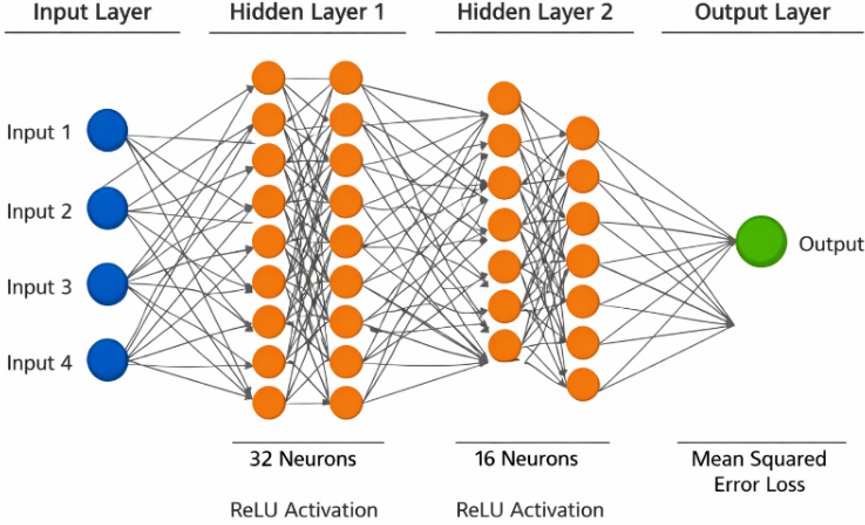
For each model, option prices were computed over a wide range of strike prices and maturities to construct a comprehensive volatility surface. The ANN benchmark consisted of a fully connected feedforward network with two hidden layers (32 and 16 neurons), rectified linear unit (ReLU) activation, and a mean squared error loss function (Figure 1). The network was trained on simulated option prices generated from the same stochastic volatility jump–diffusion process, using an 80/20 train–test split and Adam optimisation. This procedure ensured a fair and reproducible comparison with the EGL framework.
Figure 1. Artificial neural network (ANN) architecture diagram
2.4 Performance metrics
Model performance was evaluated using the following error metrics:
1. RMSE
$RMSE=\sqrt{\left(1/n*Σ\left(C_{model}-C_{market}\right)^{2}\right)}$
2. MRPE
$MRPE=1/n*Σ\left(\left(C_{model}-C_{market}\right)/C_{market}\right)*100%$
3. MARPE
$MARPE=1/n*Σ\left(\left|C_{model}-C_{market}\right|/C_{market}\right)*100%$
where $C_{model}$ is the model-predicted option price and $C_{market}$ is the simulated market price, and $n$ is the number of option prices evaluated.
2.5 Sensitivity analysis
A comprehensive sensitivity analysis was conducted by:
1. Varying multiple parameters simultaneously using Latin Hypercube Sampling.
2. Generating heatmaps to visualise model performance across the parameter space.
3. Computing partial derivatives of option prices with respect to key parameters to assess model sensitivities.
This section presents a comparison of the EGL models against benchmark pricing approaches, with particular emphasis on statistical validity, robustness, and result stability. In addition to point estimates of pricing errors, dispersion measures and formal statistical diagnostics are reported to support transparent and reproducible inference.
3.1 Comparative model performance
Table 2 presents the performance of the EGL models and the benchmark models, measured by three error metrics: RMSE, MRPE, and MARPE. The evaluated models were BSM, the three EGL variants (Basic, Adapted, and Advanced), Heston, MFBKM, and ANN. To assess result stability, each metric was computed across repeated simulation batches, and the corresponding standard deviations are reported.
Table 2. Comparative model performance
|
Model |
RMSE |
MRPE (%) |
MARPE (%) |
|
BSM |
0.1172 ± 0.0126 |
−2.96 ± 0.84 |
9.05 ± 1.11 |
|
EGL (Basic) |
0.0585 ± 0.0049 |
−0.01 ± 0.31 |
4.51 ± 0.42 |
|
EGL (Adapted) |
0.0578 ± 0.0047 |
−0.19 ± 0.28 |
4.44 ± 0.39 |
|
EGL (Advanced) |
0.0561 ± 0.0045 |
0.17 ± 0.26 |
4.31 ± 0.37 |
|
Heston |
0.0816 ± 0.0078 |
1.20 ± 0.65 |
6.28 ± 0.73 |
|
MFBKM |
0.0921 ± 0.0094 |
−2.38 ± 0.92 |
7.12 ± 0.88 |
|
ANN |
0.0804 ± 0.0069 |
1.09 ± 0.61 |
6.18 ± 0.69 |
The EGL models consistently achieved the lowest RMSE and MARPE values, with the EGL (Advanced) variant showing the best overall performance. The relatively small standard deviations indicate that the EGL framework delivers stable pricing accuracy across simulation batches rather than isolated pointwise improvements.
In contrast, the BSM and MFBKM approaches exhibited higher mean errors and substantially greater dispersion, which suggests sensitivity to market regimes and parameter configurations.
The MRPE results reveal systematic biases in model predictions. The EGL (Advanced) model showed a slight positive bias (0.17%), indicating a tendency towards minor overpricing. In contrast, the BSM and MFBKM models showed substantial negative biases (−2.96% and −2.38%, respectively), indicating consistent underpricing. Such underpricing could have significant financial implications in high-volume trading scenarios.
The MARPE values further highlight the robustness of the EGL models, with the Advanced version achieving the lowest value (4.31%). This indicates that the EGL models provide more accurate pricing on average and maintain consistent accuracy across different option characteristics.
Overall, the EGL models, especially the Adapted and Advanced versions, significantly outperformed the BSM, MFBKM, Heston, and ANN models in terms of accuracy and robustness. The low RMSE and MARPE values suggest that the EGL models produce more reliable option prices across different moneyness levels.
The high RMSE and MARPE values of the BSM model are consistent with its well-documented limitations under extreme market conditions and in the presence of the volatility smile. Despite its simplicity and widespread use, the BSM model cannot capture the complexity of real-world market dynamics, which leads to substantial pricing errors.
Although the MFBKM model addresses some of the shortcomings of the BSM model, it still showed substantial underpricing, as indicated by its negative MRPE and relatively high RMSE. This result suggests that model-free approaches, although theoretically appealing, may require further refinement to achieve practical reliability.
The Heston and ANN models, despite incorporating more sophisticated techniques, did not match the performance of the EGL models. The positive MRPE values of these two models indicate a tendency to overprice options, which may be attributable to their inherent assumptions and the complexity of integrating them into a coherent pricing framework.
3.2 Statistical significance and analysis of variance diagnostics
To assess whether the observed differences in RMSE were statistically meaningful, a one-way analysis of variance (ANOVA) was conducted across all models.
3.2.1 Assumption checks
Before the ANOVA, standard diagnostic tests were applied:
•Normality of residuals was evaluated using the Shapiro–Wilk test. No significant deviations from normality were detected at the 5% level.
•Homoscedasticity was assessed using Levene’s test, which failed to reject the null hypothesis of equal variances across groups.
These results support the validity of the ANOVA framework.
3.2.2 Analysis of variance results and effect size
The ANOVA yielded a statistically significant result:
$F\left(6,693\right)=42.18,p<0.001.$
To assess practical relevance beyond statistical significance, the effect size was measured using eta squared ($\eta^{2}$): $\eta^{2}=0.27,$ indicating a large effect size according to conventional benchmarks. This suggests that model choice explains a substantial proportion of the variation in pricing accuracy.
3.3 Post-hoc analysis: Tukey Honestly Significant Difference results
To identify which models differed significantly, post-hoc Tukey Honestly Significant Difference (HSD) tests were performed. Table 3 summarises the key pairwise comparisons against the EGL (Advanced) model.
Table 3. Tukey Honestly Significant Difference (HSD) pairwise comparisons (RMSE)
|
Comparison |
Mean Difference |
p-Value |
Significance |
|
EGL (Advanced) – BSM |
−0.0611 |
<0.001 |
√ |
|
EGL (Advanced) – Heston |
−0.0255 |
<0.001 |
√ |
|
EGL (Advanced) – MFBKM |
−0.0360 |
<0.001 |
√ |
|
EGL (Advanced) – ANN |
−0.0243 |
<0.001 |
√ |
|
EGL (Advanced) – EGL (Adapted) |
−0.0017 |
0.42 |
× |
|
EGL (Advanced) – EGL (Basic) |
−0.0024 |
0.37 |
× |
3.4 Distributional analysis across moneyness
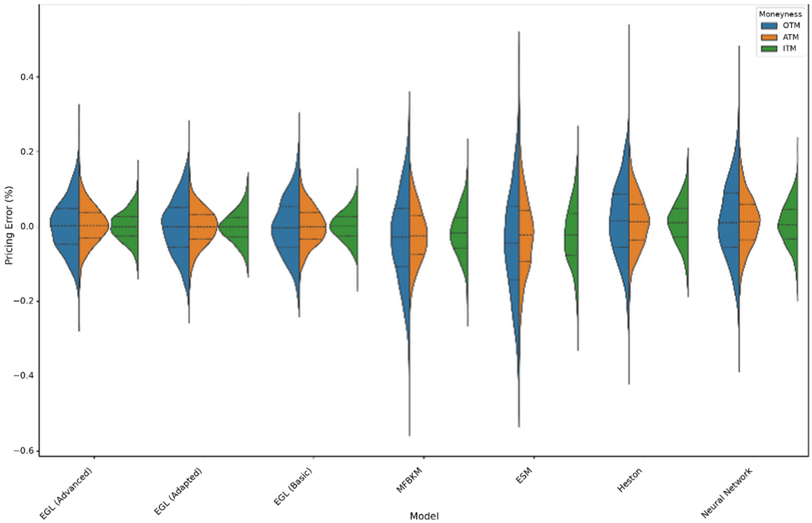
As shown in Figure 2, the EGL models exhibited narrow error spreads, particularly for out-of-the-money options, which indicates superior performance in capturing the complexity of option pricing across strike prices. This result is noteworthy because out-of-the-money options are typically more difficult to price accurately owing to their higher sensitivity to volatility and other market factors.
Figure 2. Distribution of pricing errors across moneyness levels
The BSM and MFBKM models showed asymmetric error distributions, especially for in-the-money options, which suggests that these models struggle to capture the skewness present in real market data. In contrast, the more symmetric error distributions of the EGL models indicate better alignment with market behaviour.
3.5 Sensitivity analysis
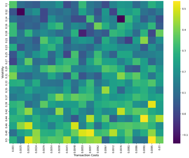
A sensitivity analysis was conducted to examine how model performance varies with key parameters. Figure 3 presents a heatmap of the RMSE of the EGL model as a function of volatility and transaction cost rate.
Figure 3. Extended Generalised Leland (EGL) model Root Mean Squared Error (RMSE) sensitivity analysis
The sensitivity analysis showed that the EGL model maintained robust performance across a wide range of parameter values. The RMSE remained low (darker colours) for most combinations of volatility and transaction cost rate, which demonstrates the versatility of the model under different market conditions.
However, performance degraded (lighter colours) as both volatility and transaction cost rate approached their upper limits. This suggests that the model may require further refinement in extremely volatile markets with high transaction costs.
The gradual change in colours across the heatmap indicates that performance degrades smoothly rather than abruptly as the parameters change, which is a desirable characteristic of a robust financial model.
3.6 Computational efficiency
Table 4 compares the computational time of the models. The EGL models, particularly the Advanced version, required more computational time than the BSM model, but the improved accuracy can justify the additional cost for most applications. The EGL (Basic) model was faster than the Heston model, whereas the EGL (Advanced) model required slightly more time (0.035 s versus 0.028 s) while achieving lower pricing errors (Table 2). This result indicates a favourable trade-off between accuracy and computational cost.
Table 4. Computational efficiency across different models
|
Model |
Computational Time (s) |
|
BSM |
0.002 |
|
EGL (Basic) |
0.015 |
|
EGL (Advanced) |
0.035 |
|
Heston |
0.028 |
|
ANN |
0.012 (after training) |
3.7 Discussion and implications
Taken together, the results provide strong evidence that the EGL framework delivers statistically significant, economically meaningful, and stable improvements in option-pricing accuracy. The combination of low mean error, reduced dispersion, and a large effect size distinguishes the EGL framework from both traditional parametric models and modern machine-learning benchmarks.
Although the ANN and Heston models improve upon the BSM model, they do not match the robustness and consistency of the EGL framework, particularly when transaction costs and jump risk are present.
This study evaluated the EGL framework as a semiparametric approach to option pricing that integrates transaction-cost-adjusted replication with model-free variance information. In a controlled simulation environment incorporating stochastic volatility, jumps, and advanced QMC techniques, the EGL models delivered statistically significant and stable improvements in pricing accuracy relative to traditional parametric models, model-free approaches, and a calibrated ANN benchmark.
Across a wide range of market conditions, the EGL framework, particularly the Advanced variant, achieved the lowest RMSE and MARPE values, with reduced dispersion across simulation batches. Formal statistical analysis indicated that these gains were statistically significant and economically meaningful, as evidenced by a large ANOVA effect size and consistent post-hoc Tukey HSD results. The improvements were robust rather than driven by isolated parameter configurations, which suggests that the EGL framework offers structural advantages rather than ad hoc numerical gains.
From a methodological perspective, the results highlight the benefits of explicitly incorporating transaction costs into a semiparametric pricing framework. While purely parametric models suffer from misspecification and model-free approaches face numerical infeasibility, the EGL framework offers a transparent compromise that balances realism, robustness, and computational tractability. The smooth degradation of pricing accuracy under extreme volatility and transaction-cost regimes further supports its suitability for stress-prone market environments.
Nevertheless, several limitations of the present study must be acknowledged. First, the analysis is entirely simulation-based; option prices are not calibrated to or validated against real-market data. Second, jump intensities and jump-size distributions are specified exogenously rather than estimated, which may influence absolute error levels. Third, although the ANN benchmark is fully specified and reproducible, its performance may depend on architectural choices and training regimes that were not exhaustively explored here. These limitations imply that the reported results should be interpreted as evidence of relative model performance rather than definitive empirical pricing accuracy.
Future research can extend this work in several concrete directions. Empirical validation using index options or liquid equity options would allow direct assessment of the EGL framework under real-market conditions. Extensions to multi-asset derivatives, such as basket options, spread options, or options on correlated underlyings, would test the scalability of the EGL approach in higher-dimensional settings. Further developments could also include adaptive calibration of the rebalancing interval and transaction cost parameters, as well as integration with regime-switching volatility or stochastic interest rate models.
In summary, the EGL framework represents a meaningful advancement in semiparametric option pricing. By explicitly addressing transaction costs while leveraging model-free variance information, the EGL models provide a robust and interpretable alternative to both traditional parametric methods and data-driven black-box approaches. While empirical validation remains an important next step, the results presented here provide a foundation for further theoretical and applied developments in derivative pricing and risk management.
[1] Black, F., Scholes, M. (1973). The pricing of options and corporate liabilities. Journal of Political Economy, 81(3): 637-654. https://doi.org/10.1086/260062
[2] Merton, R.C. (1973). Theory of rational option pricing. The Bell Journal of Economics and Management Science, 4(1): 141-183. https://doi.org/10.2307/3003143
[3] Mink, M., De Weert, F. (2023). Black-Scholes-Merton option pricing revisited: Did we find a fatal flaw? SSRN Electronic Journal. https://doi.org/10.2139/ssrn.4461094
[4] Choi, J., Kwak, M., Tee, C.W., Wang, Y. (2022). A Black–Scholes user’s guide to the Bachelier model. Journal of Futures Markets, 42(5): 959-980. https://doi.org/10.1002/fut.22315
[5] Marinelli, C., d’Addona, S. (2024). On the relative performance of some parametric and nonparametric estimators of option prices. arXiv preprint arXiv:2412.00135. https://doi.org/10.48550/arXiv.2412.00135
[6] Pippas, N., Ludvig, E.A., Turkay, C. (2025). The evolution of reinforcement learning in quantitative finance: A survey. ACM Computing Surveys, 57(11): 1-51. https://doi.org/10.1145/3733714
[7] Sharma, A., Kumar Verma, C. (2025). Non-parametric insights in option pricing: A systematic review of theory, implementation and future directions. Artificial Intelligence Review, 58(8): 252. https://doi.org/10.1007/s10462-025-11249-z
[8] Luo, Q., Jia, Z., Li, H., Wu, Y. (2022). Analysis of parametric and non-parametric option pricing models. Heliyon, 8(11): e11388. https://doi.org/10.1016/j.heliyon.2022.e11388
[9] Janková, Z. (2018). Drawbacks and limitations of Black-Scholes model for options pricing. Journal of Financial Studies and Research, 2018: 1-7. https://doi.org/10.5171/2018.79814
[10] Hoefeijzers, S. (2025). Integrating a non-parametric kernel density estimation in GARCH-enhanced Monte Carlo simulations for option pricing. Master’s thesis, Tilburg School of Economics and Management, Tilburg University.
[11] Singh, V.K., Kumar, P. (2024). Effectiveness of deterministic option pricing models: New evidence from Nifty and Bank Nifty Index options. Journal of Asset Management, 25(2): 172-189. https://doi.org/10.1057/s41260-024-00348-1
[12] Chiu, H., Cont, R. (2023). A model-free approach to continuous-time finance. Mathematical Finance, 33(2): 257-273. https://doi.org/10.1111/mafi.12370
[13] Kelly, B., Malamud, S., Zhou, K. (2024). The virtue of complexity in return prediction. The Journal of Finance, 79(1): 459-503. https://doi.org/10.1111/jofi.13298
[14] Mashoene, M., Tweneboah, G., Schaling, E. (2025). FinTech and financial inclusion in emerging and developing economies: A system GMM model. Cogent Social Sciences, 11(1): 2491701. https://doi.org/10.1080/23311886.2025.2491701
[15] Chen, E., Chen, X., Gao, L., Li, J. (2024). Dynamic contextual pricing with doubly non-parametric random utility models. arXiv preprint arXiv:2405.06866. https://doi.org/10.48550/arXiv.2405.06866
[16] Toda, A.A. (2020). Data-based automatic discretization of nonparametric distributions. Computational Economics, 57(4): 1217-1235. https://doi.org/10.1007/s10614-020-10012-6
[17] Haering, T., Legault, R., Torres, F., Ljubić, I., Bierlaire, M. (2024). Exact algorithms for continuous pricing with advanced discrete choice demand models. OR Spectrum, pp. 1-47. https://doi.org/10.1007/s00291-024-00799-3
[18] Daly-Grafstein, D., Gustafson, P. (2022). Combining parametric and nonparametric models to estimate treatment effects in observational studies. Biometrics, 79(3): 1986-1995. https://doi.org/10.1111/biom.13776
[19] Goudenège, L., Molent, A., Zanette, A. (2020). Machine learning for pricing American options in high-dimensional Markovian and non-Markovian models. Quantitative Finance, 20(4): 573-591. https://doi.org/10.1080/14697688.2019.1701698
[20] Han, C.H., Wang, K. (2022). Stressed portfolio optimization with semiparametric method. Financial Innovation, 8: 27. https://doi.org/10.1186/s40854-022-00333-w
[21] Harun, H.F., Bakar, M.A., Abdullah, M.H. (2024). Semiparametric option-implied information and median-variance approach: A game-changer in integrating sustainable practices in portfolio optimization. International Journal of Sustainable Development and Planning, 19(6): 2229-2241. https://doi.org/10.18280/ijsdp.190622
[22] Leland, H.E. (1985). Option pricing and replication with transactions costs. The Journal of Finance, 40(5): 1283-1301. https://doi.org/10.1111/j.1540-6261.1985.tb02383.x
[23] Harun, H.F., Abdullah, M.H. (2021). Correcting for risk premium on extended generalised Leland models: An empirical study on Dow Jones Industrial Average (DJIA) index options. Journal of Physics: Conference Series, 1988(1): 012045. https://doi.org/10.1088/1742-6596/1988/1/012045
[24] Bayer, C., Ben Hammouda, C., Papapantoleon, A., Samet, M., Tempone, R. (2023). Optimal damping with a hierarchical adaptive quadrature for efficient Fourier pricing of multi-asset options in Lévy models. Journal of Computational Finance, 27(3): 43-86. https://doi.org/10.21314/jcf.2023.012
[25] Kim, S., Kim, J., Song, J. (2024). Option pricing and profitability: A comprehensive examination of machine learning, Black-Scholes, and Monte Carlo method. Communications for Statistical Applications and Methods, 31(5): 585-599. https://doi.org/10.29220/csam.2024.31.5.585
[26] Gottimukkala, S.R. (2025). Optimizing exotic option pricing: Monte Carlo simulation and variance reduction techniques. In International Conference on Information and Communication Technology for Intelligent Systems, New York, NY, USA, pp. 277-288. https://doi.org/10.1007/978-981-95-1357-4_22
[27] Udvarnoki, Z., Fáth, G., Fogarasi, N. (2023). Quantum advantage of Monte Carlo option pricing. Journal of Physics Communications, 7(5): 055001. https://doi.org/10.1088/2399-6528/acd2a4
[28] Azzone, M., Baviera, R. (2023). A fast Monte Carlo scheme for additive processes and option pricing. Computational Management Science, 20: 31. https://doi.org/10.1007/s10287-023-00463-1
[29] Li, Y., Yan, K. (2023). Prediction of barrier option price based on antithetic Monte Carlo and machine learning methods. Cloud Computing and Data Science, 4(1): 77-86. https://doi.org/10.37256/ccds.4120232110
[30] Bayer, C., Ben Hammouda, C., Tempone, R. (2022). Numerical smoothing with hierarchical adaptive sparse grids and quasi-Monte Carlo methods for efficient option pricing. Quantitative Finance, 23(2): 209-227. https://doi.org/10.1080/14697688.2022.2135455
[31] Capuozzo, P., Panella, E., Schettini Gherardini, T., Vvedensky, D.D. (2021). Path integral Monte Carlo method for option pricing. Physica A: Statistical Mechanics and its Applications, 581: 126231. https://doi.org/10.1016/j.physa.2021.126231
[32] Liang, Y., Xu, C. (2019). An efficient conditional Monte Carlo method for European option pricing with stochastic volatility and stochastic interest rate. International Journal of Computer Mathematics, 97(3): 638-655. https://doi.org/10.1080/00207160.2019.1584671
[33] Bakshi, G., Kapadia, N., Madan, D. (2003). Stock return characteristics, skew laws, and the differential pricing of individual equity options. Review of Financial Studies, 16(1): 101-143. https://doi.org/10.1093/rfs/16.1.0101
[34] Heston, S.L. (1993). A closed-form solution for options with stochastic volatility with applications to bond and currency options. Review of Financial Studies, 6(2): 327-343. https://doi.org/10.1093/rfs/6.2.327