
Renny Eka Putri* | Rio Afandi | Omil Charmyn Chatib | Darius El Pebrian | Ashadi Hasan
© 2026 The authors. This article is published by IIETA and is licensed under the CC BY 4.0 license (http://creativecommons.org/licenses/by/4.0/).
OPEN ACCESS
Effective soil management requires timely information on field variability and changing soil conditions. This study presents an Internet of Things (IoT)-enabled instrumentation system for real-time, in-situ measurement of soil electrical conductivity (EC) in maize cultivation, supporting the United Nations Sustainable Development Goals (SDG 2: Zero Hunger and SDG 13: Climate Action). The system integrates soil EC sensors embedded directly in the field and connected to an ESP32 microcontroller via the Modbus RS485 communication protocol, ensuring reliable field operation. Field experiments were conducted across four cultivation plots during three cultivation phases: before planting, after the first fertilization, and after the second fertilization. Sensor performance, communication reliability, and spatial variability of soil EC were evaluated. Spatial EC distribution was analyzed using Kriging (a geostatistical interpolation method), while maize growth was assessed through periodic plant height measurements and analyzed using analysis of variance (ANOVA) and correlation analysis. The results revealed spatial and temporal variation in measured soil EC across the study plots, with changes observed following fertilizer application. Correlation analysis showed a positive association between measured EC and maize growth at the observed growth stages (r = 0.79 at 30 days after planting (DAP) and r = 0.72 at 45 DAP). These results indicate that the proposed IoT-based system can provide georeferenced, in-situ EC measurements and spatial visualization of field variability. The system therefore provides a means of monitoring changes in soil EC under field conditions and generating information that may support further assessment of site-specific soil management. However, fertilizer-use efficiency, crop yield improvement, nutrient losses, economic benefits, and greenhouse gas emissions were not directly measured in this study and cannot be established from the present results.
Internet of Things, maize, precision agriculture, soil electrical conductivity, soil nutrient monitoring, spatial analysis, Sustainable Development Goals
Precision agriculture aims to manage a farm by utilizing advanced technology to monitor and assess land and crops and adjust the treatment according to the land and crop conditions. Precision agriculture uses spatial and temporal information to characterize variability within agricultural fields and to support management decisions based on observed field conditions. Technologies such as sensing, remote monitoring, geospatial analysis, and variable-rate application can provide information needed to better understand and manage this variability. Moreover, the projected increase in global food demand associated with population growth toward 9–10 billion by 2050 has encouraged the adoption of technologies such as the Internet of Things (IoT), remote sensing, and variable-rate application in agriculture [1, 2]. These technologies are increasingly used to improve the management of agricultural resources while accounting for variability within cultivated areas. Spatial variability is an important consideration in precision agriculture because differences in soil and crop conditions can be used to identify areas requiring different management practices [3-5].
Corn (Zea mays L.) is not only consumed widely by humans and animals but also exploited in various industrial fields. Therefore, there is a high demand for its yields and productivity [6, 7]. The more yields and productivity are achieved, the more nutrients are needed in the soil to outgrow the plants. As shown in several studies, the use of NPK fertilizer has successfully increased the number of the yields [8-10]. Soil electrical conductivity (EC) can be used as an indirect proxy for the concentration of dissolved ions in the soil, which is influenced by multiple factors such as moisture, temperature, and salinity. Soil EC is a useful proxy for characterizing soil physicochemical conditions and can provide information related to salinity, soil moisture, and dissolved-ion dynamics [11, 12]. However, its interpretation as an indicator of nutrient availability or soil fertility requires consideration of other soil properties and site-specific conditions.
Many farmers merely use fertilizer without adjusting it to the soil conditions in some areas. Occasionally, they only observe the plant condition manually in determining to use fertilizer. This indeed impacts the harvest [13]. The assessment of the nutrient content of soil can only be done scientifically in a laboratory by analyzing soil samples. Undoubtedly, it requires funds and allocated time. Furthermore, the samples do not immediately cover a larger area; as a result, it is nearly impossible to obtain high spatial accuracy data [14-16]. In other words, laboratory analysis cannot be the sole indicator for determining the type and amount of fertilizer for the soil [17, 18].
The real-time monitoring of soil EC serves as a vital approach for understanding the dynamic changes in the soil environment while supporting more sustainable agricultural management. Soil EC is influenced by dissolved salt content, moisture levels, soil texture, and other physicochemical characteristics; consequently, it acts as an indicator for identifying spatial and temporal variations in soil conditions and potential salinity risks [19, 20]. Continuous EC monitoring enables the rapid detection of soil condition changes related to nutrient movement, salt accumulation, and irrigation processes, allowing water and fertilizer application to be adjusted to actual field conditions. Real-time monitoring of soil EC provides information on spatial and temporal changes in soil conditions. Soil EC is influenced by dissolved ions, soil water content, temperature, texture, and other physicochemical properties [19, 20]. Consequently, repeated EC measurements can be used to characterize changes in field conditions over time and to identify spatial patterns that may be relevant to subsequent soil and crop assessment. When integrated with georeferenced measurements, EC monitoring can provide a spatial basis for evaluating field variability and supporting further soil management analysis. Thus, integrating real-time EC monitoring with precision agriculture technologies can provide additional spatial and temporal information for characterizing field variability and supporting subsequent soil-management assessment [19, 20]. This study additionally supports SDG 2 (Zero Hunger) through the provision of field-scale insights that can refine soil and fertilizer management, and SDG 13 (Climate Action) by allowing for ongoing georeferenced assessments of soil EC, which can assist in recognizing variations in soil conditions related to fertilizer application and rainfall variability.
This has prompted the adoption of sensing technologies to obtain timely information on soil conditions and nutrient-related indicators. The technology facilitates the development of an instrumentation system for measuring soil EC in situ and obtaining spatially referenced EC data under field conditions. The system is also able to manage the spatial variability by integrating geographic coordinates from a Global Positioning System (GPS) module. The resulting georeferenced measurements can subsequently be processed in a Geographic Information System (GIS) to visualize the spatial distribution of measured soil EC. The integration of soil sensing, GPS-based georeferencing, and IoT data acquisition enables EC measurements to be associated with specific sampling locations and displayed as spatial information. Such measurements can be used to characterize field variability and temporal changes in soil EC during crop cultivation. Based on this approach, the present study aimed to develop an IoT-enabled instrumentation system for in-situ soil EC measurement and to evaluate its performance for monitoring the spatial and temporal variability of EC in a maize field. Therefore, this study aimed to develop an IoT-driven instrumentation system and then do an assessment to its use by testing the soil EC in a real-time setting.
The study was conducted in Ulakan. It is a district in Pariaman Regency of West Sumatra, Indonesia, located at coordinates of 0°40'49"S and 100°10'31"E. The instruments were assembled, and the data were processed in the Instrumentation and Control Laboratory, Department of Agricultural and Biosystems Engineering, Faculty of Agricultural Technology, Andalas University.
2.1 Design of soil electrical conductivity measurement prototype
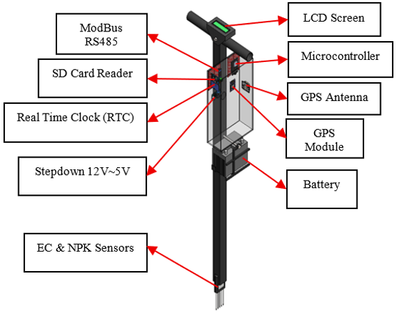
The prototype was designed as a portable, efficient, and user-friendly tool to be used in assessing soil EC more accurately and promptly. The mechanical design of the prototype was designed taking into account portability, ease of use (ergonomics), and durability in the field environment. This design can be seen in Figure 1.
Figure 1. Computer-aided design (CAD) of electrical conductivity (EC) measuring instrument prototype
The main structure of the tool consists of five main parts, namely:
a. Handle: Designed in a 'T' shape to provide a sturdy and comfortable grip for the user. This shape allows the user to apply steady vertical pressure when the probe is inserted into the ground. On the handle, an LCD screen is also placed as an output interface for the user.
b. Frame: The frame is a vertical iron rod that forms the backbone of the tool where the component housing and battery are placed.
c. Component Container: In the middle of the frame, a transparent container (box) is installed, which functions to accommodate and protect all electronic circuits, such as the microcontroller, sensor module, and battery, from exposure to dust, moisture, and physical impact.
d. Sensor: Located at the bottom end of the tool, consisting of five stainless steel metal rods designed to be tapered. The pointed tip makes it easy to penetrate into various types of soil textures. Stainless steel was chosen because it is conductive, strong, and resistant to corrosion, thereby ensuring measurement accuracy and tool durability.
e. Battery: The battery is a unit that supplies power (power supply) to all components that require electrical energy to run. AVRLA battery with 5 Ah capacity is used so that it can supply power for longer and is easy to recharge for reuse.
2.2 Control system design for soil electrical conductivity measurement instrument
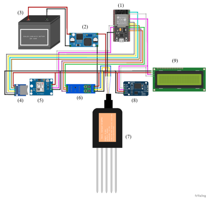
The design of the control system aims to regulate how each electronic component works together for data acquisition, processing, and storage. This system is designed based on the ESP32 microcontroller, which acts as a central processing unit. This control system integrates 6 main modules: 7-in-1 soil sensor, GPS module, real-time clock (RTC) module, SD card module, LCD, and power supply (battery). Each module has specific functions that are coordinated by the ESP32 to produce comprehensive data (Figure 2).
Details of the functionality and configuration of each component in the control system are as follows:
a. ESP32 microcontroller
As the brain of the system, the ESP32 microcontroller plays a central role in orchestrating all tool operations. It is also mainly responsible for processing raw data from soil nutrient sensors, recording time accuracy from the RTC module, and retrieving geographic coordinate data from the GPS module. Afterward, the ESP32 compiles all of those into a single structured record, which is then permanently stored on the SD card for upcoming analysis.
b. 7-in-1 soil sensor
The soil parameters were measured using a 7-in-1 soil sensor with an RS485 Modbus-RTU communication interface. The sensor simultaneously measures soil moisture, temperature, EC, pH, nitrogen (N), phosphorus (P), and potassium (K). According to the sensor technical manual, the measurement ranges are 0–100% for soil moisture, −40 to 80 ℃ for soil temperature, 0–10 mS/cm for EC, 3–9 for pH, and 0–1,999 mg/kg for N, P, and K. The corresponding accuracies are ±3% for moisture within 0–53% and ±5% within 53–100%, ±0.5 ℃ for temperature, ±0.3 for pH, and ±2% full scale for N, P, and K, while the reported resolutions are 0.10% for moisture, 0.1 ℃ for temperature, 10 mS/cm for EC, 0.01 for pH, and 1 mg/kg for N, P, and K. The sensor operates through an RS485 Modbus-RTU interface, has an IP68 protection rating, and a response time of less than 1 s. The main input component is a 7-in-1 soil sensor that measures EC, N, P, K, soil moisture, temperature, and pH. The sensor needs to be connected to the ESP32 through an RS485 interface with a converter module in order to enable it to be linked to the microcontroller. On the sensor, pins A and B must be connected to the converter module, which then converts and transmits data signals to the digital pins on the ESP32 for the analysis process.
c. DS3231 real-time clock module
To ensure the accuracy of the time log for each measurement data, a DS3231 RTC module is integrated into the system, as this module consistently records highly precise time in seconds, minutes, hours, and even the date.
d. Global Positioning System module
To provide geographic location data (geotagging) at every soil sampling location, the system requires integration with the GPS module in order to retrieve signals from satellites, which can then accurately determine latitude and longitude coordinates.
e. Secure digital card module
Data is permanently stored in the secure digital (SD) card module. It stores any data, e.g., sensor values, time, and coordinates that have been collected and processed by the ESP32. The data is saved in file formats of ‘.txt’ or ‘.csv’ for subsequent access and analysis using software such as Microsoft Excel or GIS tools. The connection of this module to the ESP32 is done through the SPI (Serial Peripheral Interface) communication protocol, with the CS pin connected to GPIO 5, SCK to GPIO 18, MISO to GPIO 19, and MOSI to GPIO 23.
f. Liquid crystal display
This system is installed with a 16 × 2 liquid crystal display (LCD) module, integrated with an I2C driver. The driver significantly simplifies the wiring process due to the use of only two data lines to connect the ESP32 and the display. The SDA (Serial Data) pin must be connected to GPIO 21, and the SCL (Serial Clock) pin must be connected to GPIO 22, allowing the LCD module to be connected to the ESP32 using the I2C protocol. The power supply for this LCD module is taken from the output connection on the step-down and GND on the ESP32. This screen will later function to display various sensor measurement values in real-time.
g. Power supply (battery)
To ensure portability and operational capability in the field, the entire system is designed to be powered by a 12 V battery. However, since the ESP32 microcontroller and most sensors operate at a much lower voltage, a step-down converter module is required. In this design, an LM2596 module is used to step down the input voltage from 12 V to a stable 5 V output voltage. The positive output (OUT+) of the LM2596 module is then connected to the 5 V VIN pin on the ESP32 board, while the negative output (OUT-) is connected to the GND pin. The positive output from the power supply will be used by other components as a more stable power source than directly from the ESP32, and the negative output of all components is connected to the same ground, including the GND of the ESP32.
h. System integration with Google Spreadsheet
The system utilizes Google Apps Script as a bridge between the ESP32 microcontroller and Google Spreadsheet to implement real-time data storage to the cloud. The connection mechanism is done through an API endpoint created by publishing Apps Script as a web app. First, a special script is written within the Google Spreadsheet environment that functions to receive web requests. A unique URL with the data is generated by Google when the script is successfully published. Meanwhile, on the device, once the ESP32 is connected to the Wi-Fi network, it retrieves all the information. Subsequently, the microcontroller converts the data to URL format and then sends it through a request of an HTTP GET to the particular URL of the web application. Running the designated function, extracting the data parameter from the incoming requests, and applying the ‘appendRow()’ function to input the data as a new row in the spreadsheet are done by the Google Apps Script. This secures and organizes that every measurement is promptly recorded in the Google Spreadsheet.
2.3 Field experimental conditions and measurement procedure
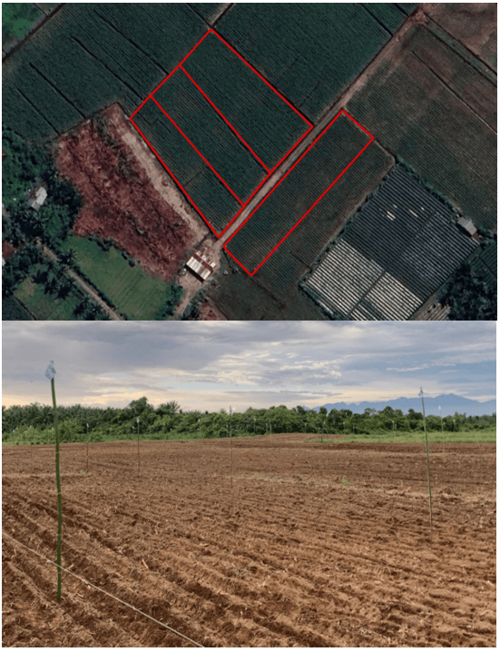
The field experiment was conducted in Ulakan District, Pariaman Regency, West Sumatra, Indonesia, at coordinates 0°40'49"S and 100°10'31"E. The experimental field consisted of four maize cultivation plots. Plots 1, 2, and 3 were managed using predetermined NPK fertilizer applications, with dimensions of 18 m × 79 m, 20.2 m × 79 m, and 18 m × 79 m, respectively. Plot 4 measured 25 m × 85 m and was managed according to the conventional practices of local farmers, including farmer-applied fertilizer without intervention from the researchers. The plots were separated by irrigation ditches, as shown in Figure 3, which functioned as irrigation channels for water distribution within the field.
Figure 3. Land for performance testing
The experimental soil was characterized by dark-colored, slightly sandy soil containing residual maize plant materials and manure from previous cultivation. Initial soil properties were characterized through laboratory analysis of two soil samples collected from the experimental field. The analyzed properties included soil water content, total nitrogen (N-total), available phosphorus (P₂O₅), exchangeable potassium (K-dd), organic carbon (C-organic), and the C/N ratio. The results of the initial soil analysis are presented in Table 1. In addition to the laboratory analysis, baseline soil EC was measured at the established sampling points and spatially represented using ordinary Kriging.
Table 1. Initial soil properties based on laboratory analysis
|
Soil Property |
Sample 1 |
Sample 2 |
|
Water content (%) |
7.86 |
6.71 |
|
Total N (%) |
0.64 |
0.75 |
|
Available P₂O₅ (ppm) |
17.66 |
10.04 |
|
Exchangeable K (cmol/kg) |
0.15 |
0.17 |
|
Organic C (%) |
4.09 |
3.84 |
|
C/N ratio |
6.39 |
5.12 |
The maize used in the experiment was a hybrid feed maize cultivar, NK 7328 BtGT, a biotech maize hybrid developed by Syngenta. NPK fertilizer with an N-P₂O₅-K₂O composition of 16-16-16 was applied to Plots 1–3 at planting and at 35 days after planting (DAP), with different application rates among the plots. The fertilizer application rates and management conditions for each experimental plot are presented in Table 2. Plot 4 was managed according to the local farmer's conventional practice and received fertilizer from the farmer without intervention from the researchers.
Table 2. NPK fertilizer application for each experimental plot
|
Plot |
Application at Planting (kg/ha) |
Application at 35 DAP (kg/ha) |
Total (kg/ha) |
|
Plot 1 |
200 |
300 |
500 |
|
Plot 2 |
150 |
200 |
350 |
|
Plot 3 |
100 |
100 |
200 |
|
Plot 4 |
* |
* |
* |
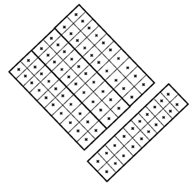
Three EC observation phases were conducted: (1) baseline measurement before the first NPK fertilizer application, (2) measurement after the first NPK application at planting, and (3) measurement after the second NPK application at 35 DAP. Twenty sampling points were established within each plot, resulting in a total of 80 sampling points across the four plots. The same sampling points were revisited during each observation phase. At each sampling point, one EC reading was recorded per phase, and no repeated readings were taken at the same sampling point within a single phase. The sensor probe was inserted vertically into the soil to a depth of 6.6 cm, corresponding to the length of the probe. The measured EC value, geographic coordinates, and measurement time were recorded for subsequent spatial and temporal analysis.
The study area has a humid tropical climate characterized by relatively high temperature, humidity, and rainfall throughout the year. Climatic conditions in Padang Pariaman during 2025 were characterized by frequent rainfall events, including episodes of heavy rainfall, as indicated by BMKG daily climate records for the region [21]. Such humid conditions and rainfall variability are relevant to soil EC measurements because changes in soil water content can affect the concentration and movement of soluble ions and consequently influence measured soil EC. Therefore, climatic conditions were considered an important environmental factor when interpreting the spatial and temporal variation of soil EC in the experimental field.
Calibration of the EC measurement was performed by comparing the readings of the developed 7-in-1 Modbus RS485 soil sensor with those obtained from a YY-1080 6-in-1 Soil Tester operating in EC mode. Both instruments were positioned at the same georeferenced sampling locations and measurements were conducted simultaneously to minimize differences in soil conditions between the two measurements. A total of 10 paired EC measurements were used for the calibration analysis. The paired measurements were analyzed using linear regression to establish the calibration relationship between the developed sensor and the reference instrument. The coefficient of determination (R²) was used to evaluate the strength of the linear relationship, while root mean square error (RMSE) and mean absolute error (MAE) were used to quantify the differences between the sensor and reference measurements. The resulting regression equation was subsequently applied to correct the raw EC readings obtained from the developed sensor before further spatial and statistical analyses. The treatment for planting the corn underwent three different phases: (1) prior to planting and first fertilization, (2) after the first fertilization, and (3) after the second fertilization. At each sampling point, one EC reading was recorded during each observation phase. No repeated readings were taken at the same sampling point within a single observation phase. Changes in measured EC across the three phases were subsequently evaluated (Figure 4).
Figure 4. Land plots and data collection points
2.4 Observations and data analysis
Twenty sampling points were established within each plot, resulting in 80 sampling points across the four plots. The same sampling points were revisited during each of the three observation phases. At each point, a single EC reading was collected per phase, resulting in 80 EC observations for each phase and 240 point-phase observations across the three phases. The raw EC readings obtained from the developed sensor were corrected using the calibration equation established from the reference-instrument comparison. The corrected EC values were subsequently used for Kriging interpolation and statistical analysis. A univariate analysis of variance (ANOVA) was performed to examine variations in measured soil EC associated with crop age, fertilizer dosage, sampling point, and the interaction between crop age and fertilizer dosage. The significance level was set at 0.05. Because each fertilizer dosage was represented by one field plot, the sampling points within each plot were treated as observations rather than independent experimental replicates for evaluating fertilizer treatment effects. Therefore, treatment-related findings were interpreted as exploratory differences among the monitored plots rather than definitive causal effects of fertilizer dosage.
Spatial interpolation of soil EC was performed using ordinary Kriging in ArcGIS ArcMap 10.8. The EC measurements were georeferenced using the WGS 1984 UTM Zone 47S coordinate reference system. For each plot and observation phase, 20 georeferenced sampling points were used to generate the corresponding interpolated EC map. The same sampling locations were revisited during each observation phase. The variogram was fitted automatically by the software, and the final nugget, sill, and range parameters were obtained from the fitted variogram model rather than manually specified. A variable search radius was used with a maximum of 12 neighboring points and one search sector. The search neighborhood was circular.
To examine the association between measured soil EC and plant growth, the EC data were compared with plant growth parameters, particularly plant height and number of leaves. The analysis was conducted to examine whether spatial variation in measured soil EC was associated with variation in plant growth. The effect of soil EC on plant growth was monitored periodically at 30 and 45 DAP, covering the period from the vegetative to the generative stage. The observations were mainly on the height, number of leaves, width of leaves, and stem diameter. The data from these observations were analyzed to examine the association between soil EC and plant growth using Pearson correlation analysis, comparing EC values with plant-growth variables (height, number of leaves, leaf width, and stem diameter). This has been employed by previous studies, indicating that EC in soil can contribute to plant growth, and EC spatial interpolation combined with physiological data of the plant can provide insight into proper management of farming. The sensor-generated EC data were obtained by calculating the descriptive statistics (mean, standard deviation, coefficient of variation), while the plant growth data illustrated dominant tendencies and variability. Combining Kriging mapping, ANOVA, and correlation analysis provided an analytical framework for evaluating sensor performance, spatial and temporal variability in measured soil EC, and its association with plant growth.
3.1 Sensor calibration
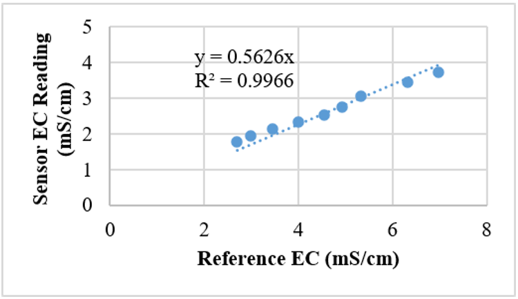
The calibration analysis was performed using 10 paired EC measurements obtained from the developed sensor and the YY-1080 reference instrument. The measurements covered the observed EC range of the calibration dataset. The results showed a strong linear relationship between the reference EC measurements and the readings obtained from the developed sensor, with a regression equation of y = 0.5626x and R² of 0.9966 (Figure 5). In this relationship, x represents the reference EC value, and y represents the raw EC reading obtained from the developed sensor. Because the regression equation expresses the sensor reading as a function of the reference measurement, the equation was rearranged to obtain the reference-equivalent EC value from the raw sensor reading. Accordingly, the corrected EC value was calculated by dividing the raw sensor reading by 0.5626. The corrected EC values were then used in the subsequent spatial and statistical analyses. The RMSE and MAE obtained from the calibration dataset were 2.102 mS/cm and 1.963 mS/cm, respectively. These metrics were calculated using the same 10 paired measurements used to establish the linear regression equation and therefore represent the calibration-fit errors rather than independent validation errors. The results indicate the magnitude of the differences between the sensor-derived EC values and the reference measurements within the calibration dataset. However, because an independent dataset was not used for validation, these results do not establish the accuracy or generalizability of the developed sensor under other soil and environmental conditions. Further validation using independent measurements and laboratory-based EC analysis is required.
The calibration assessment was based on 10 paired field measurements and comparison with a reference field instrument. Therefore, the results should be interpreted within the EC conditions represented by the calibration dataset. The calibration procedure did not constitute independent laboratory validation of the sensor. Further validation using laboratory-based EC measurements and a broader range of soil and environmental conditions would be required to establish the general measurement accuracy of the sensor. There was a strong correlation between EC and capacitance-based sensors and the concentrations of dissolved nutrient ions, with R² values between 0.97 and 0.99 [22]. The Modbus RS485 sensor demonstrated stable performance throughout the study, requiring less frequent recalibration despite potential electrical noise and interference. These findings are consistent with those reported in a previous study [23], which also demonstrated the effectiveness of the sensor for EC measurement. Therefore, it was confirmed that the EC sensor was reliable to be used as an integrative parameter in the real-time monitoring of soil EC.
Figure 5. Calibration relationship between the developed sensor and the reference electrical conductivity (EC) instrument
3.2 Real-time monitoring of electrical conductivity levels
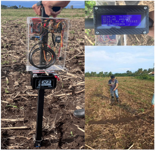
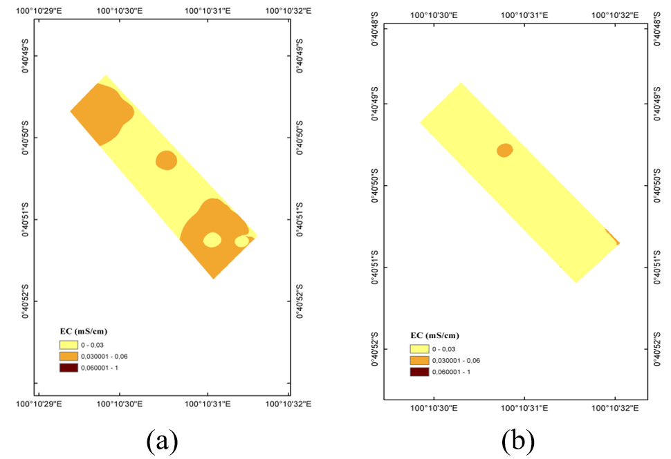
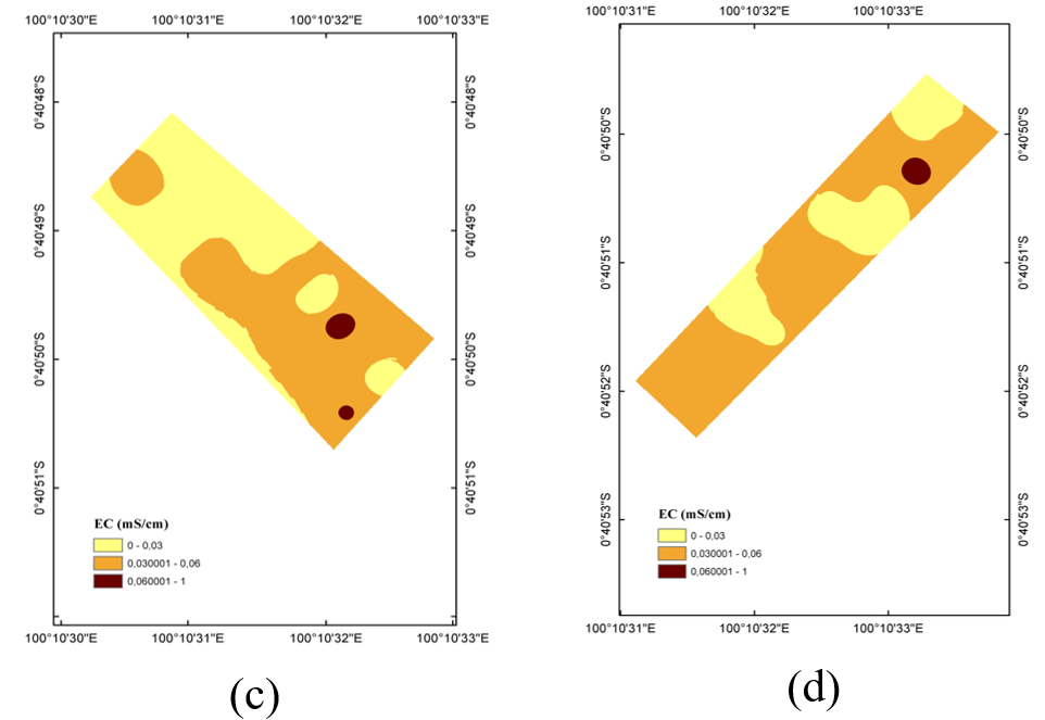
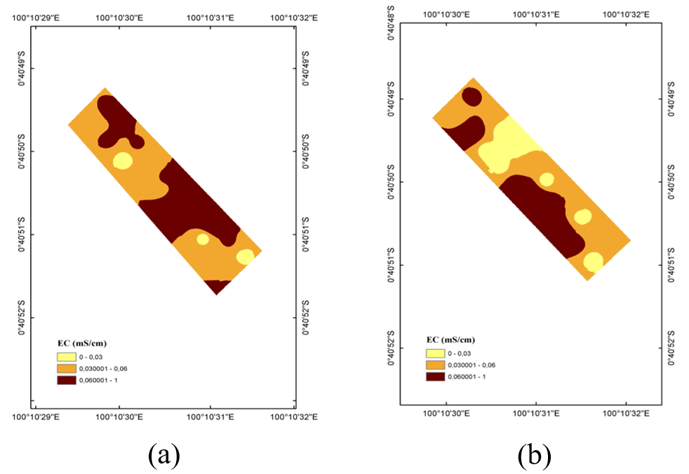
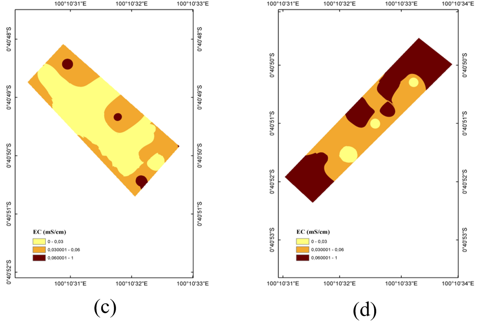
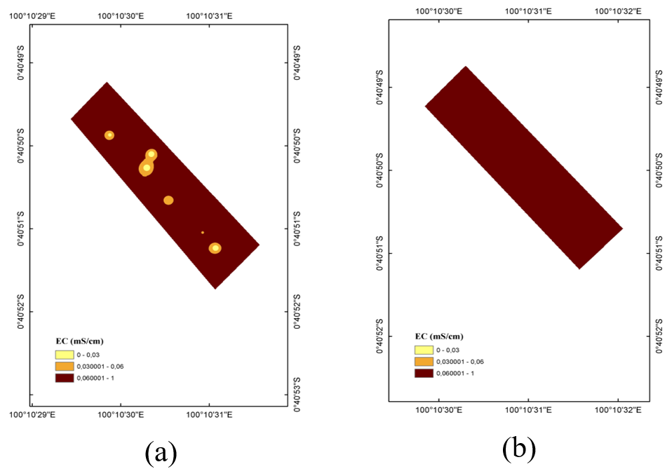
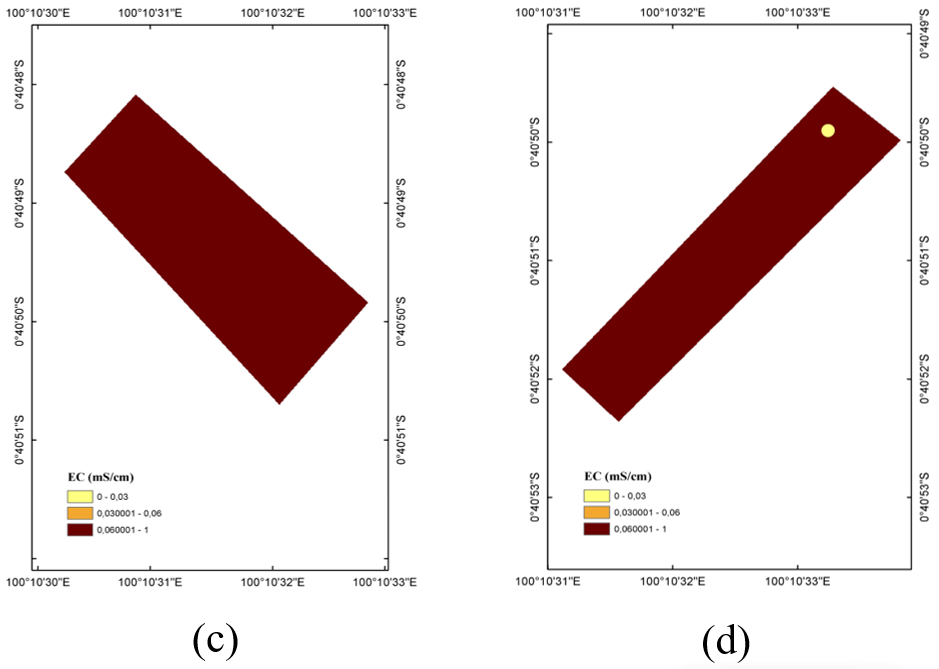
A real-time monitoring of soil EC was able to retrieve thorough spatial data of the soil. The georeferenced EC measurements provided spatial data for characterizing field variability. The data were processed using Kriging interpolation to visualize the distribution of measured EC across the study plots and cultivation phases. These spatial patterns were used to describe changes in EC before and after fertilization and to examine the variability observed among sampling locations. The resulting maps provide spatial information that can support subsequent assessment of soil conditions and field management (Figure 6). The data collection became the basis for the spatial analysis of the EC distribution. The Kriging interpolation technique helped to generate the map estimation of the overall EC value throughout the study sites. The measured EC value was visually indicated by the color gradient representing low (light yellow), medium (orange), and high (dark brown) EC classes. This observation covered four research plots (plot 1, plot 2, plot 3, and plot 4) throughout 3 phases of corn planting: prior to planting, after the first fertilization, and after the second fertilization (Figures 7–9).
Figure 6. Field installation of the Internet of Things (IoT)-based electrical conductivity (EC) measurement system
Spatial interpolation of soil EC was performed using ordinary Kriging in ArcGIS ArcMap 10.8. The EC measurements were georeferenced using the WGS 1984 UTM Zone 47S coordinate reference system. For each plot and observation phase, 20 georeferenced sampling points were used to generate the corresponding interpolated EC map. The same sampling locations were revisited during each observation phase. The experimental variogram was automatically fitted using a spherical model. The final nugget, sill, and range parameters were obtained from the fitted variogram model rather than specified manually. A variable search radius was used with a maximum of 12 neighboring points and one search sector. The search neighborhood was circular. The selected variogram model and its fitted parameters are reported in Table 3. The performance of the Kriging interpolation was assessed using cross-validation. Prediction performance was evaluated using mean error (ME), RMSE, mean standardized error (MSE), and root mean square standardized error (RMSSE).
Cross-validation was performed using 80 observations. The ME was 0.00037 mS/cm, while the RMSE was 0.0296 mS/cm. The MSE was 0.0136, and RMSSE was 0.978. The RMSSE value close to 1 indicates that the estimated prediction uncertainty was broadly consistent with the observed prediction errors. The regression slope of 0.1003 indicates a smoothing effect; therefore, the interpolated EC maps should be interpreted as representations of spatial patterns rather than exact point values. The interpolated EC maps should be interpreted as representations of spatial patterns rather than exact point values.
Table 3. Variogram parameters and cross-validation results of ordinary Kriging for soil electrical conductivity (EC) interpolation
|
Parameter |
Value |
|
Nugget (mS/cm²) |
0 |
|
Sill (mS/cm²) |
0.000967 |
|
Major range (decimal degrees) |
0.000166 |
|
Major range (approx., m) |
18.5 |
|
Mean error (ME) |
0.00037 |
|
Root mean square error (RMSE) |
0.0296 |
|
Mean standardized error (MSE) |
0.0136 |
|
Root mean square standardized error (RMSSE) |
0.978 |
In the pre-fertilization phase, the EC distribution was heterogeneous. Unlike plot 2, which was dominated by low EC levels, plots 1, 3, and 4 showed spatial variability across low, medium, or high EC levels. The observed pattern indicates that the measured EC distribution was heterogeneous across the plots. However, after the first treatment in the fertilizing process, the number of EC values rose significantly across all plots. Notable shifts were found mostly in plots 1, 2, and 4, where the conductivity areas were in more medium (orange) and high (dark brown) levels, particularly in plot 2, which was at a low value once and then promptly shifted to the medium EC level. The measured EC values were higher in several plots after the first fertilization phase than in the pre-fertilization maps.
A further change in measured EC was observed following the second fertilization treatment, with higher EC values recorded across the study plots. All four plots displayed a dominant dark brown coverage, which indicated that they were in the highest range of EC level. This coincided with broader areas of higher measured EC across the study-site maps. Because each fertilizer dosage was represented by a single plot and other soil and environmental factors were not independently controlled, the observed spatial changes cannot be attributed solely to fertilizer application. The soil EC patterns across the four plots showed noticeable temporal and spatial variation across the fertilization phases and were also influenced by intrinsic spatial heterogeneity. The pre-fertilization maps showed predominantly low measured EC values in several areas, represented by the light-yellow gradient. These patterns indicate spatial variation in EC rather than directly indicating low nutrient concentrations. This phenomenon is in accordance with what the literature suggests: soil texture, moisture, and residual nutrient salts are the main factors influencing EC values [24]. Due to differences in soil chemical composition or moisture retention, plot 1 and plot 3, before fertilization, exhibited a moderately higher level of EC. This confirmed that the site was not uniformly homogeneous, aligning with typical spatial heterogeneity found in farming soil.
Following the first fertilization, a broader distribution of moderate EC values was observed in the Kriging maps. This change may reflect changes in dissolved-ion conditions associated with fertilization, although the specific chemical changes were not directly measured in this study. The observed spatial pattern after fertilization was consistent with the formation of spatially distinct EC zones, with the observed distribution potentially reflecting differences in soil moisture, ionic composition, texture, and field management [25]. Unlike plots 1 to 3, plot 4 was cultivated traditionally, which displayed a more variable level of EC compared to the other plots, which may reflect inconsistencies in traditional farmer fertilization methods [26].
The IoT-based EC sensor captured changes in the spatial distribution of measured EC across the study sites, with greater variation observed after the fertilization phases. The most substantial increase in all plots was shown after the second fertilization phase, as the gradient of darker brown can be seen across the map. This observation was consistent with the temporal change in measured EC following repeated fertilization [27]. The EC levels were more consistent and moderate in plots 1 and 2, indicating that fertilization was performed regularly and uniformly. Meanwhile, EC levels in plot 4 were much higher, as it was expected, since the spatial pattern of EC in plot 4 was more heterogeneous, which may reflect differences in field management and underlying soil conditions [28]. High EC values may reflect differences in soil properties such as moisture conditions, texture, organic matter, and microtopography; however, these factors were not independently evaluated in the present study [29].
The 3-phase observation revealed changes in the spatial distribution of measured EC from lower to higher EC classes across the observation periods. These changes may reflect temporal variation in dissolved-ion conditions, soil moisture, and other site factors; however, the specific chemical changes were not directly measured in this study. These changes were effectively captured and shown by the Kriging interpolation method, which is consistent with former studies that have reported the suitability of Kriging for characterizing the spatial variability of soil-related properties [30]. The three-phase observations also showed that the spatial distribution of measured EC was not uniform across the study plots, reflecting spatial heterogeneity in the observed field conditions. These findings support the use of precision agriculture technologies for obtaining spatial information that may assist further field and soil-management assessment [31]. Overall, integrating in-situ EC sensing with geostatistical analysis provides a practical approach for characterizing the spatial variability of measured soil EC. The resulting information can be used as supporting data for further evaluation of field conditions within a precision agriculture framework.
3.3 Changes in measured soil electrical conductivity across fertilization phases
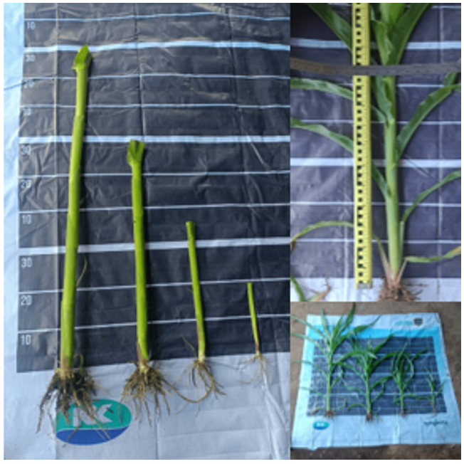
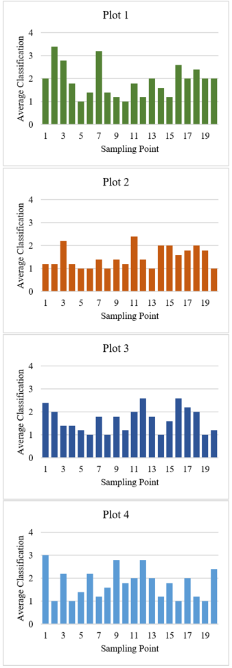
Corn growth was classified by identifying the parameters after data collection. Each planting phase had a single classification system, which was performed at 30 and 45 DAP (Tables 4 and 5). Subsequently, the data from each phase were presented in the form of a bar graph, illustrating the crop growth during the observation. EC reflects the capacity of the soil environment to conduct electrical current and is affected by dissolved ions, soil moisture, texture, temperature, and other physicochemical properties. Therefore, changes in EC were analyzed as changes in measured soil conditions rather than as direct measurements of nutrient availability. The analysis was conducted to examine changes in measured EC across the different fertilization phases (Figures 7–9). Table 6 presents the ANOVA results for measured soil EC under variations in crop age, fertilizer dosage, and sampling point (Figure 10). The table also shows that plant age is the most influential factor, as it has the highest F-value (156.219; p < 0.001). The interaction of plant age and fertilizing treatment comes second (F = 5.144; p = 0.002), followed by the fertilizer treatment itself (F = 4.087; p = 0.008). On the other hand, there is no significant difference in the EC value for the sampling point factor (p = 0.682). In two growth periods, data were collected: 30 DAP and 45 DAP (Table 7). The variables of corn growth were categorized into 2 indicators: plant growth at 30 DAP (PG30) and plant growth at 45 DAP (PG45) (Figure 11).
Table 4. Classification of plant growth parameters at 30 days after planting (DAP)
|
Tall Trunk (cm) |
Stem Diameter (cm) |
Number of Leaves (Sheet) |
Leaf Width (cm) (Middle) |
Category |
Classification |
|
69–86 |
2.8 |
7 |
9.5 |
Superior |
4 |
|
52–69 |
2.5 |
7 |
9.3 |
Normal |
3 |
|
35–52 |
1.6 |
5 |
6.1 |
Currently |
2 |
|
18–35 |
0.7 |
5 |
3.6 |
Low |
1 |
In the exploratory ANOVA, there was a statistically significant crop-age term (F = 156.219, p < 0.001), fertilizer-dosage term (F = 4.087, p = 0.008), and an interaction term of crop age and fertilizer dosage (F = 5.144, p = 0.002), while the sampling-point term was not statistically significant (F = 0.819, p = 0.682). The statistically significant fertilizer-dosage variable captures differences in recorded soil EC for the observed fertilizer-dosage plots in the exploratory model. However, this finding cannot be taken as evidence for a replicated effect of the fertilizer treatment, as there was only one plot per fertilizer application. The interaction of crop age and fertilizer dosage should also be considered a pattern associated with exploratory plots rather than a direct causal effect of fertilizer.
Table 5. Classification of plant growth parameters at 45 days after planting (DAP)
|
Tall Trunk (cm) |
Stem Diameter (cm) |
Number of Leaves (Sheet) |
Leaf Width (cm) (Middle) |
Category |
Classification |
|
146–178 |
3 |
11 |
10.7 |
Superior |
4 |
|
118–146 |
2.5 |
10 |
10.3 |
Normal |
3 |
|
90–118 |
2.3 |
8 |
10 |
Currently |
2 |
|
62–90 |
2.1 |
7 |
9.6 |
Low |
1 |
Table 6. Summary of exploratory analysis of variance (ANOVA) for measured soil electrical conductivity (EC) by fertilizer dosage, plant age, and sampling point
|
Variation Sources |
Sum of Squares |
df |
Mean Square |
F |
p-Value |
|
Crop Age |
1.072 |
1 |
1.072 |
156.219 |
<0.001 |
|
Fertilizer Dosage |
0.084 |
3 |
0.028 |
4.087 |
0.008 |
|
Interaction of Crop Age and Fertilizer Dosage |
0.106 |
3 |
0.035 |
5.144 |
0.002 |
|
Sampling Point |
0.107 |
19 |
0.006 |
0.819 |
0.682 |
Figure 10. Corn plant measurement for classification
Table 7. Correlation coefficient for soil electrical conductivity (EC) and corn plant growth
|
Parameter |
Sample Size (n) |
Correlation Coefficient (r) |
p-Value |
Remarks |
|
PG30–EC |
80 |
0.79 |
0.001 |
Significant |
|
PG45–EC |
80 |
0.72 |
0.004 |
Significant |
Figure 11. Average plant classification at 30 days after planting (DAP) per plot of land
These results suggest that soil EC varied with plant age and fertilizer treatment, while the relationship between fertilizer treatment and EC depended on plant age. However, the results should be interpreted cautiously because each fertilizer treatment was applied to only one plot. Therefore, treatment effects cannot be separated from plot-specific characteristics, and the sampling points within each plot should not be considered independent experimental replicates. The analysis is consequently interpreted as exploratory evidence of differences among the monitored plots rather than as definitive evidence of causal fertilizer effects.
The correlation analysis revealed a strong positive relationship between soil EC and maize plant growth at both observation stages. At 30 DAP, the correlation coefficient was r = 0.79 (p = 0.001, n = 80), while at 45 DAP, the correlation coefficient was r = 0.72 (p = 0.004, n = 80). Both correlations were statistically significant. However, correlation does not imply causation. Other environmental and agronomic factors, including soil moisture, temperature, sunlight exposure, soil texture, and pH, may also influence plant growth and were not independently evaluated in this study. EC should be considered as one of several soil-condition indicators associated with maize growth rather than as a direct determinant of plant growth. Further research is recommended, including the study of additional environmental factors and direct analysis of soil chemistry, to determine the causal mechanisms behind the observed correlation between EC and growth.
The spatial EC mapping, plant-growth classification, exploratory ANOVA, and correlation analysis collectively characterize the spatial and temporal variation in measured soil EC and its association with maize growth. The Kriging-based interpolation showed changes in measured EC patterns across the observation phases, while the exploratory ANOVA identified crop age and fertilizer dosage as statistically significant terms within the model. However, because each fertilizer dosage was represented by a single plot, the fertilizer-related statistical results are interpreted as exploratory differences among the monitored plots rather than as replicated treatment effects. The correlation analysis further showed a positive association between measured EC and maize growth at 30 and 45 DAP.
It should be noted that soil EC is not a direct measure of nutrient availability but rather an indirect proxy influenced by multiple factors, including soil moisture content, temperature, salinity, soil texture, and the concentration of dissolved ions [24]. Corwin and Lesch [19] emphasized that apparent soil EC should be interpreted through its correlation with specific soil properties at a given site, since the same EC value can result from different combinations of salinity, moisture, and texture. Consequently, a high EC value does not necessarily indicate higher nutrient availability or improved soil fertility; it may instead reflect elevated salinity or moisture conditions unrelated to nutrient content. In this study, EC measurements and the available NPK sensor readings were considered as complementary soil measurements, while plant growth observations were used as biological response indicators. However, these sensor-derived measurements were not independently validated against laboratory soil chemical analyses. In addition, since no direct soil chemical analysis (e.g., laboratory-based nutrient testing) was conducted to confirm actual nutrient concentrations, the relationship between EC, nutrient availability, and crop response reported here should be interpreted with caution. Future studies incorporating laboratory soil chemical analysis are recommended to validate and strengthen the reliability of EC-based nutrient status estimation.
This study successfully developed an IoT-based system for in-situ measurement of soil EC. The Kriging interpolation maps revealed visible spatial heterogeneity in measured EC distribution across the plots and observation phases. The exploratory ANOVA identified statistically significant terms for crop age (F = 156.219, p < 0.001), fertilizer dosage (F = 4.087, p = 0.008), and their interaction (F = 5.144, p = 0.002), whereas sampling point was not statistically significant (F = 0.819, p = 0.682). Because each fertilizer dosage was represented by only one field plot, these fertilizer-related results should be interpreted as exploratory differences among monitored plots or management regimes rather than as evidence of replicated causal fertilizer effects. The Kriging maps therefore serve primarily as a descriptive tool for visualizing spatial EC patterns. Correlation analysis showed that soil EC was positively and significantly associated with maize growth at 30 DAP (r = 0.79) and 45 DAP (r = 0.72). This relationship should be interpreted as an association rather than a direct causal relationship because plant growth is also influenced by other environmental and agronomic factors that were not independently measured.
This study has several limitations that should be acknowledged. First, the experiment was conducted on a relatively limited dataset, comprising four cultivation plots with 20 sampling points per plot at a single research site in Ulakan, Pariaman Regency, West Sumatra. Second, the findings are specific to the soil characteristics of the study site; soils with different textures, organic matter content, or baseline salinity levels may exhibit different EC behavior. Third, this study was conducted within a single growing season, and EC values are sensitive to seasonal factors such as rainfall intensity, ambient temperature, and irrigation regime. Fourth, the EC–growth relationship established in this study is specific to maize; other crop species may respond differently to the same EC conditions. Consequently, the present study does not provide direct evidence of changes in soil nutrient concentrations or fertilizer-use efficiency. Crop yield improvement, economic benefits, nutrient losses, and greenhouse gas emissions were also not evaluated. These outcomes therefore remain beyond the scope of the present study and require separate experimental assessment. Overall, integrating EC monitoring with spatial visualization provides useful information for characterizing field variability and may support further assessment of site-specific soil management.
The authors gratefully acknowledge the financial support provided by the Directorate of Research, Technology, and Community Service (DRTPM), Directorate General of Higher Education, Research, and Technology, Ministry of Education, Culture, Research, and Technology of the Republic of Indonesia, through the Fundamental-Regular Research Scheme, under Research Contract No. 87/UN16.19/PT.01.03/PL/2025, Fiscal Year 2025. The authors also gratefully acknowledge the financial support for the presentation of this research at the international conference provided by the Indonesian Endowment Fund for Education (LPDP), on behalf of the Ministry of Higher Education, Science and Technology of the Republic of Indonesia, and managed under the EQUITY Program, Contract No. 4304/B3/DT.03.08/2025.
|
EC |
electrical conductivity |
|
R2 |
coefficient of determination |
|
r |
Pearson correlation coefficient |
|
F |
F-statistic |
|
p |
probability value |
|
df |
degrees of freedom |
|
x |
reference EC value |
|
y |
sensor-measured EC value |
|
Subscripts |
|
|
30 |
observation at 30 days after planting |
|
45 |
observation at 45 days after planting |
|
PG |
plant growth |
|
30 |
observation at 30 days after planting |
[1] Karunathilake, E.M.B.M., Le, A.T., Heo, S., Chung, Y.S., Mansoor, S. (2023). The path to smart farming: Innovations and opportunities in precision agriculture. Agriculture, 13(8): 1593. https://doi.org/10.3390/agriculture13081593
[2] Soussi, A., Zero, E., Sacile, R., Trinchero, D., Fossa, M. (2024). Smart sensors and smart data for precision agriculture: A review. Sensors, 24(8): 2647. https://doi.org/10.3390/s24082647
[3] Groß, J., Gentsch, N., Boy, J., et al. (2023). Influence of small-scale spatial variability of soil properties on yield formation of winter wheat. Plant and Soil, 493(1-2): 79-97. https://doi.org/10.1007/s11104-023-06212-2
[4] Zhang, N., Wang, M., Wang, N. (2002). Precision agriculture—A worldwide overview. Computers and Electronics in Agriculture, 36(2–3): 113-132. https://doi.org/10.1016/S0168-1699(02)00096-0
[5] Sishodia, R.P., Ray, R.L., Singh, S.K. (2020). Applications of remote sensing in precision agriculture: A review. Remote Sensing, 12(19): 3136. https://doi.org/10.3390/rs12193136
[6] Shiferaw, B., Prasanna, B.M., Hellin, J., Bänziger, M. (2011). Crops that feed the world 6. Past successes and future challenges to the role played by maize in global food security. Food Security, 3(3): 307-327. https://doi.org/10.1007/s12571-011-0140-5
[7] Erenstein, O., Jaleta, M., Sonder, K., Mottaleb, K., Prasanna, B.M. (2022). Global maize production, consumption and trade: trends and R&D implications. Food Security, 14(5): 1295-1319. https://doi.org/10.1007/s12571-022-01288-7
[8] Wang, N., Ai, Z., Zhang, Q., et al. (2024). Impacts of nitrogen (N), phosphorus (P), and potassium (K) fertilizers on maize yields, nutrient use efficiency, and soil nutrient balance: Insights from a long-term diverse NPK omission experiment in the North China Plain. Field Crops Research, 318: 109616. https://doi.org/10.1016/j.fcr.2024.109616
[9] Setiyono, T.D., Walters, D.T., Cassman, K.G., Witt, C., Dobermann, A. (2010). Estimating maize nutrient uptake requirements. Field Crops Research, 118(2): 158-168. https://doi.org/10.1016/j.fcr.2010.05.006
[10] Hirel, B., Tétu, T., Lea, P.J., Dubois, F. (2011). Improving nitrogen use efficiency in crops for sustainable agriculture. Sustainability, 3(9): 1452-1485. https://doi.org/10.3390/su3091452
[11] Najdenko, E., Lorenz, F., Dittert, K., Olfs, H.W. (2024). Rapid in-field soil analysis of plant-available nutrients and pH for precision agriculture—A review. Precision Agriculture, 25: 3189-3218. https://doi.org/10.1007/s11119-024-10181-6
[12] Rhoades, J.D., Raats, P.A.C., Prather, R.J. (1976). Effects of liquid-phase electrical conductivity, water content, and surface conductivity on bulk soil electrical conductivity. Soil Science Society of America Journal, 40(5): 651-655. https://doi.org/10.2136/sssaj1976.03615995004000050017x
[13] Nurdin, L., Rukka, H., Kaharuddin, K. (2024). Aplikasi beberapa rekomendasi pemupukan dan dampaknya terhadap pertumbuhan dan produksi jagung pulut (Zea mays ceratina L.). Jurnal Agrisistem, 19(2): 95-101. https://doi.org/10.52625/j-agr.v19i2.296
[14] Wetterlind, J., Stenberg, B., Söderström, M. (2008). The use of near infrared (NIR) spectroscopy to improve soil mapping at the farm scale. Precision Agriculture, 9(1-2): 57-69. https://doi.org/10.1007/s11119-007-9050-0
[15] Stenberg, B., Viscarra Rossel, R.A., Mouazen, A.M., Wetterlind, J. (2010). Visible and near infrared spectroscopy in soil science. Advances in Agronomy, 107: 163-215. https://doi.org/10.1016/S0065-2113(10)07005-7
[16] Viscarra Rossel, R.A., Behrens, T., Ben-Dor, E., et al. (2016). A global spectral library to characterize the world's soil. Earth-Science Reviews, 155: 198-230. https://doi.org/10.1016/j.earscirev.2016.01.012
[17] Kuang, B., Mahmood, H.S., Quraishi, M.Z., Hoogmoed, W.B., Mouazen, A.M., van Henten, E.J. (2012). Sensing soil properties in the laboratory, in situ, and on-line: A review. Advances in Agronomy, 114: 155-223. https://doi.org/10.1016/B978-0-12-394275-3.00003-1
[18] Adamchuk, V.I., Hummel, J.W., Morgan, M.T., Upadhyaya, S.K. (2004). On-the-go soil sensors for precision agriculture. Computers and Electronics in Agriculture, 44(1): 71-91. https://doi.org/10.1016/j.compag.2004.03.002
[19] Corwin, D.L., Lesch, S.M. (2003). Application of soil electrical conductivity to precision agriculture: Theory, principles, and guidelines. Agronomy Journal, 95(3): 455-471. https://doi.org/10.2134/agronj2003.4550
[20] Corwin, D.L., Scudiero, E. (2020). Field-scale apparent soil electrical conductivity. Soil Science Society of America Journal, 84(5): 1405-1441. https://doi.org/10.1002/saj2.20153
[21] Badan Meteorologi, Klimatologi, dan Geofisika (BMKG). (2025). Southeast Asian Climate Assessment & Dataset (SACA&D): Daily climate data, sacad.bmkg.go.id, accessed on June 14, 2026
[22] Sudduth, K.A., Kitchen, N.R., Bollero, G.A., Bullock, D.G., Wiebold, W.J. (2003). Comparison of electromagnetic induction and direct sensing of soil electrical conductivity. Agronomy Journal, 95(3): 472-482. https://doi.org/10.2134/agronj2003.4720
[23] Kitchen, N.R., Sudduth, K.A., Myers, D.B., Drummond, S.T., Hong, S.Y. (2005). Delineating productivity zones on claypan soil fields using apparent soil electrical conductivity. Computers and Electronics in Agriculture, 46(1-3): 285-308. https://doi.org/10.1016/j.compag.2004.11.012
[24] Corwin, D.L., Lesch, S.M. (2005). Apparent soil electrical conductivity measurements in agriculture. Computers and Electronics in Agriculture, 46(1-3): 11-43. https://doi.org/10.1016/j.compag.2004.10.005
[25] Vanninen, I., Pereira-Querol, M., Engeström, Y. (2015). Generating transformative agency among horticultural producers: An activity-theoretical approach to transforming Integrated Pest Management. Agricultural Systems, 139: 38-49. https://doi.org/10.1016/j.agsy.2015.06.003
[26] Aubert, B.A., Schroeder, A., Grimaudo, J. (2012). IT as enabler of sustainable farming: An empirical analysis of farmers' adoption decision of precision agriculture technology. Decision Support Systems, 54(1): 510-520. https://doi.org/10.1016/j.dss.2012.07.002
[27] Rhoades, J.D., Chanduvi, F., Lesch, S. (1999). Soil salinity assessment: Methods and interpretation of electrical conductivity measurements. FAO Irrigation and Drainage Paper 57. https://www.fao.org/4/x2002e/x2002e.pdf.
[28] Basso, B., Fiorentino, C., Cammarano, D., Schulthess, U. (2016). Variable rate nitrogen fertilizer response in wheat using remote sensing. Precision Agriculture, 17: 168-182. https://doi.org/10.1007/s11119-015-9414-9
[29] Brevik, E.C., Calzolari, C., Miller, B.A., et al. (2016). Soil mapping, classification, and pedologic modeling: History and future directions. Geoderma, 264(Part B): 256-274. https://doi.org/10.1016/j.geoderma.2015.05.017
[30] Webster, R., Oliver, M.A. (2008). Geostatistics for Environmental Scientists (2nd ed.). Wiley.
[31] Gebbers, R., Adamchuk, V.I. (2010). Precision agriculture and food security. Science, 327(5967): 828-831. https://doi.org/10.1126/science.1183899