
Asmaa Abdul-Razzaq Al-Qaisi* | Enas Muzaffer Jamel | Qutaiba J Altai | Raghad Abdulaali Azeez
© 2026 The authors. This article is published by IIETA and is licensed under the CC BY 4.0 license (http://creativecommons.org/licenses/by/4.0/).
OPEN ACCESS
Retinal scanning is a biometric method used to identify individuals. It plays a significant role in security because each person has a unique retinal print that differs from others, just like fingerprints. In this research, we built a model to verify a person's identity using a retinal image. A retinal image is captured, and a series of treatments is applied to it, including extracting the green channel, removing noise using a Gaussian Filter, and normalizing and improving contrast using the CLAHE technique. In the next stage, segmentation is performed using the Fiber metric; in two stages, a pre-improvement stage and a post-improvement stage, the two methods are compared to extract blood vessels. This is followed by an image feature extraction process for input into the classifier. Two types of classifiers were employed in this study: EfficientNet-B0, which segments the image into patches and subsequently classifies them; and a convolutional neural network (CNN) utilizing the "Adam Optimizer." To mitigate overfitting, we incorporated the "Dropout" technique and added a "Global Average Pooling" layer before the fully connected layer to improve learning efficiency. Furthermore, data augmentation was performed to improve the network's ability to evaluate new data. Performance metrics, specifically the Dice coefficient, Area Under the Curve (AUC), sensitivity, and specificity, were calculated using the DRIVE dataset, with a learning rate of 0.001 and training durations of 20 epochs for the CNN and three epochs for EfficientNet.
classification, convolutional neural network, EfficientNet, CLAHE, segmentation, skeletonization
Each person has a unique retinal blood pattern (arteries and blood vessels) that is not repeated in another person and differs in the branching pattern of the arteries and the bends and intersections of the blood vessels. Infrared cameras are used to image these blood vessels, with images from one eye captured separately from those from the other to increase image resolution [1]. There are three main ways to distinguish the right eye from the left eye. One of these common ways is the location of the optic nerve, where the location of this nerve is on the right side of the right eye and vice versa [2]; the second method is the vascular map pattern [3]; and the third method is by tracking the location of the central arteries and veins for physiological optics [4]. Optical coherence tomography (OCT) is one of the most important techniques in medical imaging for diagnosing the retina, as it captures retinal tissue with high accuracy by focusing on the macula, which plays a major role in vision [5]. In this study [6], the superpixel algorithm has been used to segment the optic cup and calculate cup-to-disc ratio (CDR) to detect retinopathy. Several segmentation methods have also been used, such as K-means, Hough transform, and fuzzy C-mean clustering, to obtain accurate diagnostic results. Retinal images of the right and left eyes were classified by highlighting blood vessels using support vector machine (SVM). Training was done based on detection and segmentation through image processing, and an accuracy of 94.1176% was achieved [7].
In this research, a series of treatments were performed on the image by extracting the green area, removing noise, and improving contrast, then performing the image segmentation process before and after optimization, extracting features, and then training the data on a convolutional neural network (CNN) with the Adam optimizer.
The following succinctly describes this study's primary contributions:
1. For retinal image patches classified into vessel and background classes, a methodical framework for segmenting retinal vessels based on EfficientNet-B0 is created.
2. To improve vessel-related data before deep learning classification, a preprocessing pipeline including green-channel extraction, Gaussian filtering, intensity normalization, and CLAHE is incorporated.
3. To lessen the extreme imbalance between vessel and background samples, a balanced patch-generation technique is used with the DRIVE ground-truth and region-of-interest masks.
4. To prevent patches from the same retinal image from being concurrently assigned to training and validation subsets inside the same fold, an image-level 5-fold cross-validation technique is used. This offers a more trustworthy assessment of the model's capacity for generalization.
5. TP, TN, FP, FN, Accuracy, Precision, Sensitivity, Specificity, F1-score, Dice coefficient, Area Under the Curve (AUC), and Receiver Operating Characteristic (ROC) analysis, along with mean ± standard deviation across the five folds, are used to provide a thorough evaluation framework.
Network classification has attracted the attention of many researchers. While deep learning approaches automatically extract characteristics from retinal images, traditional retinal vascular segmentation methods mostly rely on manually created features and pre-established image-processing procedures. There are still issues, such as small datasets, class imbalance, and the identification of thin and low-contrast vessels, even if deep learning techniques are better able to capture intricate vessel patterns. In order to assess CNN and EfficientNet-B0's capacity to differentiate between vessel and background pixels under identical experimental conditions, this study employs a patch-based methodology.
Previous studies have investigated retinal vessel segmentation using a variety of image processing, machine learning, and deep learning techniques. Staal et al. [8] proposed a ridge-based segmentation method and achieved an accuracy of 0.944 and a sensitivity of 0.734. Marín et al. [9] employed a neural network approach, obtaining an accuracy of 0.945, a sensitivity of 0.706, and a specificity of 0.980. Fraz et al. [10] used a morphological method and reported an accuracy of 0.948, a sensitivity of 0.740, and a specificity of 0.980.
Roychowdhury et al. [11] introduced a graph-cut-based method, achieving an accuracy of 0.952, a sensitivity of 0.739, and a specificity of 0.978. Azzopardi et al. [12] proposed COSFIRE filters for retinal vessel detection and obtained an accuracy of 0.944, a sensitivity of 0.765, and a specificity of 0.970. Liskowski and Krawiec [13] applied a deep CNN, reporting an accuracy of 0.953, a sensitivity of 0.781, and a specificity of 0.980. Fu et al. [14] combined CNN with conditional random fields (CRF) and achieved an accuracy of 0.947 and a sensitivity of 0.729.
Son et al. [15] proposed a Generative Adversarial Network (GAN)-based segmentation approach, obtaining an accuracy of 0.954, a sensitivity of 0.789, and a Dice score of 0.83. Fraz et al. [16] combined matched filtering, AdaBoost, and machine learning classification, achieving an accuracy of 0.972, a sensitivity of 0.873, and a specificity of 0.988. Zhou et al. [17] proposed BTS-DSN with a deeply supervised CNN and reported an accuracy of 0.956, a sensitivity of 0.821, a specificity of 0.980, and a Dice score of 0.83. Guo et al. [18] combined Fuzzy C-means, level-set segmentation, and a hybrid machine learning approach, achieving an accuracy of 0.961, a sensitivity of 0.761, and a specificity of 0.981.
Ronneberger et al. [19] introduced the U-Net architecture for deep-learning-based segmentation and reported an accuracy of 0.956, a sensitivity of 0.796, a specificity of 0.981, and a Dice score of 0.79. Oktay et al. [20] proposed Attention U-Net and obtained an accuracy of 0.961, a sensitivity of 0.814, a specificity of 0.984, and a Dice score of 0.81. He et al. [21] employed a ResNet50-UNet architecture with transfer learning, achieving an accuracy of 0.964, a sensitivity of 0.842, a specificity of 0.983, and a Dice score of 0.80. Abràmoff et al. [22] reported a sensitivity of 0.84 and a specificity of 0.64 using a general retinal vessel segmentation algorithm.
In the present study, a CNN-based approach optimized using the Adam algorithm was investigated for retinal vessel classification. The proposed method achieved an accuracy of 0.9931 and a sensitivity of 0.99744, while the reported specificity and Dice/F1 score were 0.28089 and 0.19687, respectively. These results are included to provide a direct numerical comparison with previously reported methods; however, differences in datasets, experimental protocols, class distributions, preprocessing procedures, and evaluation criteria should be considered when interpreting the results.
Overall, the studies under examination show that no single segmentation strategy consistently achieves the best results across all evaluation metrics. While deep learning techniques can learn more representative features, they are more reliant on training data and computational resources; traditional approaches offer comparatively straightforward and computationally efficient solutions but primarily rely on manually created features. The evaluation of CNN and EfficientNet-B0 within the same experimental environment is motivated by these discrepancies.
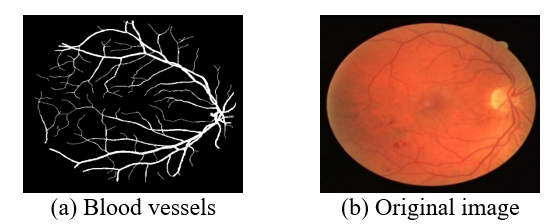
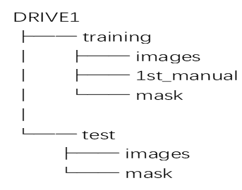
The DRIVE dataset is used; the images were acquired using a Canon CR5 camera with 80-bit color depth, a resolution of 584 × 768 pixels, and a circular field of view with a diameter of 540 pixels. A mask also indicated the area of interest and defined the field of view. The screening sample included 400 people from the general public, aged between 25 and 90 years. Forty high-resolution images were selected directly from this sample; 33 showed no signs of retinopathy, while 7 showed signs of retinopathy. These 7 images were then divided into two groups of 20 images each [23]. Figure 1 shows samples of images, and Figure 2 shows the structure of the dataset.
Figure 1. Sample of a dataset [23]
Figure 2. Structure of the dataset
3.1 Dataset division and cross-validation
There are forty retinal pictures in the DRIVE dataset. Five-fold cross-validation was used to split the photos at the image level in order to guarantee a trustworthy assessment and prevent data leakage. Eighty percent (32 photos) and twenty percent (8 images) of the images in each fold were used for training and validation, respectively. Only after the image-level division were patch extraction and augmentation carried out. The given results are presented over the five folds to provide a more comprehensive assessment of model performance, as the small number of original retinal images may impact the deep learning models' capacity for generalization.
This work presents a deep learning-based framework for segmenting retinal vessels from fundus images. In order to create a comprehensive retinal vessel map, the suggested methodology first divides local retinal image patches into two classes: vessel and backdrop. Then, it reconstructs the patch-level predictions. The approach integrates deep CNN learning with retinal-specific image preprocessing.
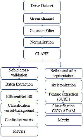
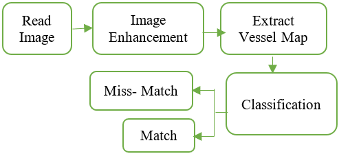
The experimental study takes into account two deep learning models. EfficientNet-B0 is utilized as the primary deep learning architecture for vessel/background patch categorization, while a traditional CNN model serves as a baseline to serve as a reference for assessing the effectiveness of the suggested method. Because of its effective architecture and capacity to extract hierarchical visual features while preserving a comparatively compact model structure, EfficientNet-B0 was chosen Figure 3 Shows the overall model.
Figure 3. The overall model
4.1 Preprocessing
At this stage, the data is optimized and prepared before training to obtain accurate results. The goal of this stage is to make the blood vessels more visible, and the following steps are included.
Step 1: Read images and extract the green channel to provide optimal contrast for vessels, reduce noise, and simplify processing, which is a preferred method for blood vessels.
Step 2: Gaussian filters are used to remove noise, and objects smaller than 50 pixels are deleted.
Step 3: normalization to transform the image so that the brightness is uniform, and a specific standard deviation is defined to reduce the difference in illumination between the right and left eyes.
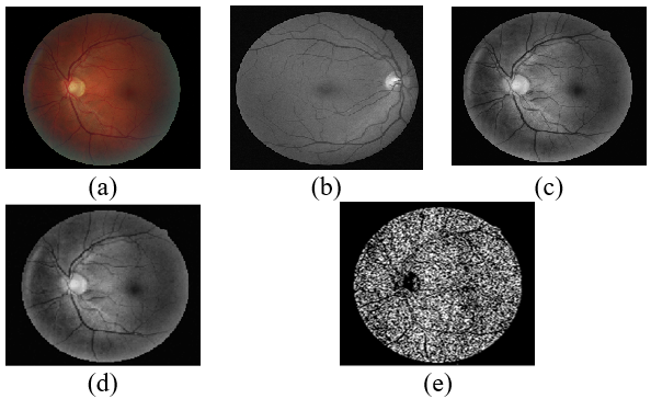
To evaluate the performance of the system, A series of improvements were made to the retinal image in Figure 4, where the original image is shown in (Figure 4(a)), to obtain results with high accuracy in discrimination. First, the green channel was extracted (Figure 4(b)), (Figure 4(c)) shows a Gaussian filter, and the lighting was improved (Figure 4(d)), then the noise was removed (Figure 4(e)(.
Figure 4. (a) Original image, (b) green channel, (c) Gaussian filter, (d) contrast enhancement, (e) noise
4.2 CLAHE algorithm
It is a technique used to improve the details of an image with varying lighting conditions, making it clearer, especially when the image is dark or contains unevenly lit areas, as shown in the following steps.
1. Divide the image into areas called tiles.
2. Apply histogram equalization to each region of the image separately.
3. Apply contrast limit to prevent noise amplification in the image.
4. Merge the areas again to obtain an improved image.
4.3 Vessel segmentation map
At this stage, the important area of the image (the retina) is identified using the standard method of extracting blood vessels through two methods:
4.3.1 Segmentation before enhancement
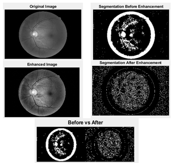
In this method, Adaptive Thresholding was used to determine the threshold for each area in the image, not the entire image, because the retinal image contains differences in illumination. The image contains dark and illuminated areas. We also determined the sensitivity of vessel detection. If it is greater than 0.55, this means detecting more vessels. However, if the value is less than 0.55, this means reducing noise and then deleting small parts in the binary image whose value is less than 50 pixels because they form light points or noise and cause a segmentation error. The steps of this method are as follows.
1. Convert the image from gray to binary
2. Adaptive Thresholding
3. Sensitivity = 0.55
4. Remove small objects from the binary image
5. Image enhancement with CLAHE
6. Fiber metric
4.3.2 Segmentation after optimization
Here, the image is converted to grayscale, i.e., converted to the standard field. Then, Sensitivity = 0.45 is used because the Vesselness image has become clearer, so we need less sensitivity to reduce noise, and then remove small components less than 50 pixels.
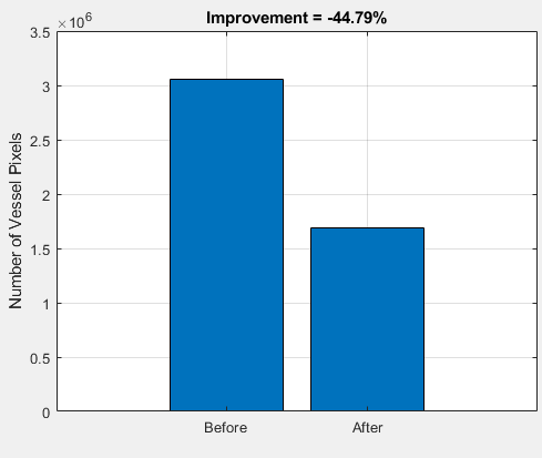
Segmentation was performed on the image in two stages. The first stage represents segmentation before optimization, and the second stage represents segmentation after optimization. Then, a comparison was made between the two methods as shown in Figure 5(a) and (b). The difference between the two stages is that, in Segmentation before enhancement, the result appears without improvement, but in the case of Segmentation after enhancement, a better result is obtained if the values are modified.
Figure 5. Comparison of the result before and after segmentation, (a) image comparison (b) graphical comparison
4.4 Skeletonization
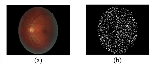
At this stage, the vessel is transformed into a thin line and used to analyze the network and extract properties, as shown in Figure 6(a) and (b).
Figure 6. Vessel transformation process: (a) Original image, (b) skeletonization
4.5 Feature extraction
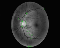
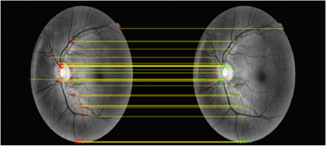
In this step, the Speeded-Up Robust Features (SURF) algorithm is used to search for distinctive points within an image, such as edges, corners, and points of significant lighting variation, and then converts these points into a digital description for comparison with another image, and saves the features in a database, as shown in Figure 7.
Figure 7. Extract retina feature
4.6 Data augmentation
In retinal images, the number of images is small, so Augmentation is done to help the model learn better by increasing the number of images, reducing the overfitting problem, and making the model more robust.
Retinal images are different due to shooting angle, lighting, and eye movement, so Data Augmentation simulates these changes.
The core idea involves partitioning the image into patches; EfficientNet-B0 then classifies these patches as either "vessel" or "background," and the resulting predictions are used to reconstruct the vessel map.
The preprocessed retinal images were divided into 64 × 64-pixel patches. Each extracted patch was subsequently resized to (224 × 224 × 3) pixels and replicated across three channels to match the input dimensions required by EfficientNet-B0.
5.1 Data partitioning and cross-validation
The 40 retinal images in the DRIVE dataset are divided into 20 training and 20 testing images. Five-fold cross-validation was used to assess the 20 training images at the image level. Four photos (20%) were utilized for validation, and sixteen images (80%) were used for model training in each fold. To prevent patches created from the same retinal image from being dispersed among the training and validation subsets, partitioning was done prior to patch extraction.
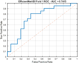
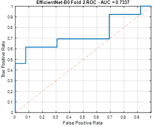
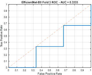
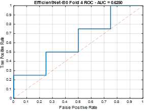
Only the final vessel-map prediction was made using the 20 original DRIVE test photos, which were kept entirely separate from the cross-validation process. Neither model validation nor training involved the usage of test images. Quantitative performance metrics were not calculated for the test set since the implemented test folder lacks the required manual vessel annotations. As a result, the five image-level validation folds yielded the accuracy, precision, sensitivity, specificity, F1-score, Dice, and AUC reported in this study, as shown in Table 1, which are then displayed as mean ± standard deviation.
Table 1. EfficientNet-B0 metrics
|
Metrics |
Fold1 |
Fold2 |
Fold3 |
Fold4 |
Fold5 |
|
Accuracy |
0.690 |
0.615 |
0.500 |
0.500 |
0.875 |
|
Precision |
0.722 |
0.600 |
0.500 |
0.500 |
0.800 |
|
Sensitivity |
0.619 |
0.692 |
0.333 |
0.750 |
1.000 |
|
Specificity |
0.761 |
0.538 |
0.666 |
0.250 |
0.750 |
|
F1-Score |
0.666 |
0.642 |
0.400 |
0.600 |
0.888 |
|
Dice |
0.666 |
0.642 |
0.400 |
0.600 |
0.888 |
|
AUC |
0.741 |
0.733 |
0.333 |
0.625 |
1.000 |
5.2 Five-fold cross-validation
Five-fold cross-validation was used to get a more accurate estimate of model performance because the DRIVE dataset has a small number of retinal images. Instead of doing cross-validation at the patch level, it was done at the retinal-image level. Five folds were randomly selected from the 20 training photos. Four images were utilized for validation, and sixteen images were used for training for each fold. The matching training and validation images were then used for independent patch extraction. As a result, the training and validation subsets did not share patches from the same retinal image.
Figure 8. EfficientNet-B0 for fold1
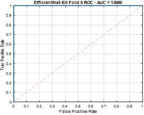
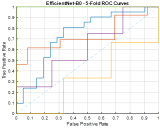
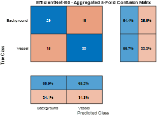
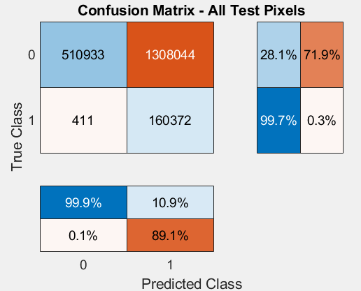
The process was repeated for each of the five folds, and the mean and standard deviation were used to summarize the performance metrics acquired from each fold. The 20 initial DRIVE test images were saved for final prediction only and were not used for cross-validation. With a vessel threshold of 0.01, if the proportion of vessel pixels within the patch is greater than or equal to 1%, the patch is classified as a vessel; otherwise, it is considered background, as shown in Figures 8-13 and the confusion matrix in Figure 14.
Figure 9. EfficientNet-B0 for fold2
Figure 10. EfficientNet-B0 for fold3
Figure 11. EfficientNet-B0 for fold4
Figure 12. EfficientNet-B0 for fold5
Figure 13. EfficientNet-B0 for all folds
Figure 14. Confusion matrix for EfficientNet-B0
At this stage, a CNN is used to learn to distinguish between vessel and background. The model is trained using a loss function that includes Dice loss and binary cross-entropy, and an optimizer (Adam).
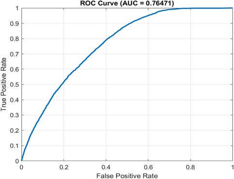
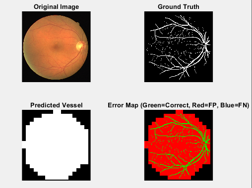
The neural network consists of three convolutional layers. The first convolutional layer uses 3 × 3 filters to detect features (edges and textures), then uses 32, 64, and 128 filters. Padding is then applied to keep the spatial size constant. Normalization works to organize values within the network to accelerate training, reduce vanishing gradient issues, and achieve higher accuracy. The nonlinear activation function (RELU) was used to enable the network to learn complex patterns. Max pooling in this layer reduces image size, minimizes computations, and utilizes key features. Figure 15 shows the AUC, and Figure 16 shows the predicted vessel.
Figure 15. Area Under the Curve (AUC) measure
Figure 16. Extract the vessel
Represents the distribution of predictions versus Ground Truth for each pixel, with rows representing the true category (Background/Vessel) and columns representing the expected category. The closer the values of the main diagonal TP, TN are to 100%, the better the performance of the model [24-26]. Table 2 shows the components of the confusion matrix, where:
The most important criteria calculated are:
Sensitivity: Represents the model's ability to detect blood vessels and is computed from Eq. (1), as shown in Table 2.
Sensitivity $=\frac{T P}{T P+F N}$ (1)
Accuracy: It measures the proportion of correct predictions out of all predictions, computed from Eq. (2).
Accuracy $=\frac{T P+T N}{T P+T N+F P+F N}$ (2)
Specificity: Represents the model's ability to distinguish the background and is computed from Eq. (3), as shown in Table 2.
Specificity $=\frac{T N}{T N+F P}$ (3)
Precision: Measures the proportion of correct positive predictions among all cases the model classifies as positive, computed from Eq. (4).
Precision $=\frac{T P}{T P+F P}$ (4)
Dice Coefficient: Represents the degree of congruence between the actual segmentation and the segmentation generated by the model. A Dice value of 1 indicates perfect agreement, while a value of 0 indicates no overlap; it is computed from Eq. (5), as shown in Table 2.
Dice $=\frac{2 x T P}{2 x T P+F P+F N}$ (5)
AUC: Measures the model's ability to truly distinguish between the two categories, Vessel and Background [27, 28].
Table 2 explains the metrics, Figure 17 shows the results, and Table 3 shows the pixel-wise confusion matrix.
Table 2. Explains the metrics
|
Metric |
Value |
|
Accuracy |
34.516 |
|
Precision |
11.146 |
|
Sensitivity |
o.99744 |
|
Specificity |
0.28089 |
|
Dice |
0.19687 |
|
F1-Score |
0.19687 |
|
AUC |
0.76471 |
Table 3. The pixel-wise confusion matrix
|
Confusion Matrix |
Kind of Evaluation |
Type of Evaluation |
Description |
|
Con.Mat. No.1 |
Training |
Network Learning |
It compares expectations with the data used in training |
|
Con.Mat. No.2 |
Patch Level |
Patch Ranking |
Comparing the model results with data not used in training, but at the 64x64 patch level, where classification is done while the Vessel or Background network is evaluated with small inputs |
|
Con.Mat. No.3 |
Pixel Level |
Final Segmentation Image |
Called pixel-wise confusion matrix, Each pixel in the real image is compared with the pixel expected by the model to evaluate the actual segmentation quality of the images, from which Sensitivity, Specificity, and Dice are calculated |
Figure 17. Output of the classifier
F1-Score: A single metric that balances precision and recall by taking their harmonic mean. When recall and precision values are similar but not identical, it is especially helpful, as explained in Eq. (6).
F1-Score $=\frac{(2 * \text { Precision } * \text { Recall })}{(\text { Precision }+ \text { Recall })}$ (6)
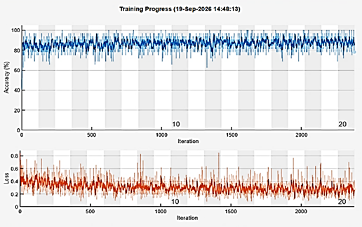
We used several complementary metrics, such as accuracy, precision, sensitivity, specificity, F1-score, Dice coefficient, and AUC, to assess the model's performance. Despite achieving a high sensitivity of 0.99744, the model's specificity was comparatively low (0.28089), suggesting that many background pixels were mistakenly identified as vessel pixels. Due to the impact of these false-positive predictions on the overlap between the projected and ground-truth vessel areas, the Dice coefficient was likewise comparatively low (0.19687). As a result, sensitivity or AUC alone should not be used to evaluate the model's performance. A more thorough understanding of the segmentation performance is offered by the confusion matrix and the full set of evaluation metrics; Figure 18 shows the training operations.
Figure 18. The training operations
This section outlines all training settings, as shown in Table 4.
Table 4. Training setting
|
Paremeter |
Convolutional Neural Network (CNN) |
EfficientNet-B0 |
|
Input patch size |
64 × 64 |
64 × 64 |
|
Network patch size |
64 × 64 × 3 |
224 × 224 × 3 |
|
Convolution stride |
1 |
Network Default |
|
Patch size |
64 |
64 |
|
Optimizer |
Adam |
Adam |
|
Initial learning rate |
1 × 10⁻⁴ |
1 × 10⁻⁴ |
|
No.of epoch |
20 |
3 |
|
Dropout |
As specified in CNN architecture |
Network Default |
To test a new person, follow these steps in Figure 19. The retinal image of the subject is processed and compared against the database, after which a notification appears indicating whether the result is a match or a non-match, as shown in Figure 20.
Figure 19. A new person's test
Figure 20. Retina matching result
For EfficientNet-B0, as seen by the high sensitivity of 0.99744, the obtained findings show that the suggested model has a good ability to detect retinal artery pixels. The comparatively poor specificity of 0.28089, however, suggests that a sizable portion of background pixels are mistakenly identified as vessels. Many false-positive predictions are produced as a result of this behavior.
Despite the great sensitivity, the Dice coefficient of 0.19687 further demonstrates that there is little overlap between the ground-truth vessel map and the anticipated vessel map. This apparent disparity is not contradictory: Dice assesses the overlap between the predicted and reference vessel regions and is impacted by both false-positive and false-negative predictions, while sensitivity measures the percentage of real vessel pixels that are recognized. Therefore, if a model over-segments the retinal background as vessels, it can achieve very high sensitivity while having a low Dice coefficient.
Because of this, sensitivity by itself should not be taken as proof of better segmentation performance. Complementary information is provided by precision, specificity, F1-score, Dice, accuracy, and AUC, all of which should be taken into account together. By clearly displaying the numbers of true-positive, true-negative, false-positive, and false-negative predictions, the confusion matrix offers more proof. As a result, these criteria are taken into account collectively in the updated study to offer a more impartial evaluation of the suggested strategy.
Handling images for diagnostic purposes requires high-resolution images, so a series of treatments is needed to obtain accurate results. In this research, we used CLAHE to make the blood vessels clearer. Skeletonization was also used to determine the topological structure, measure the length of the branches, and identify the central points. In addition, calculating the AUC is necessary because accuracy may be misleading, as the image of the retina is much larger than the blood vessels, so we may obtain high accuracy even if the model fails to extract the blood vessels; however, it measures the model's ability to truly distinguish between the two categories, Vessel and Background. ROC curve in Figure 10 displays the relationship between the positive rate(sensitivity) and the false positive rate. The model is more accurate when the curve is oriented towards the upper-right corner.
The experimental results reveal different performance characteristics between the CNN and EfficientNet-B0 models. The CNN achieved substantially higher sensitivity and AUC, indicating a strong ability to detect retinal vessels. However, its low specificity and F1-score suggest a higher rate of false-positive predictions and a less balanced classification performance. In contrast, EfficientNet-B0 achieved higher specificity, F1-score, and Dice values, indicating a better balance between vessel detection and background discrimination. Therefore, the main difference between the two models lies in their performance characteristics: CNN emphasizes vessel detection, whereas EfficientNet-B0 provides a more balanced classification between vessel and background regions.
Although the performance was quite good, in the future, several improvements could be considered that could further enhance the proposed model by increasing the number of samples to support the training process and obtaining greater network balance, as well as using other image enhancement methods, such as Morphology and Frangi Filter, and enhanced training techniques such as ResNet50 and VGG19 or VGG16.
It can also be inferred in future research that more advanced deep learning architectures and optimization strategies will be used in order to further optimize classification performance. Such methods as transfer learning with pretrained CNNs, hyperparameter optimization, and ensemble learning may be potentially beneficial in terms of accuracy and stability. Moreover, automated feature extraction and attention mechanisms can be incorporated, leading to a model that can center on informative tendencies within the images. With such enhancements, further research would assist in considerably enhancing the accuracy and efficiency of the classification system, especially when operating with complex or skewed data.
The original title of the manuscript on the use of CNN technology to detect and classify people's identities using retinal images was worked on by Dr. Asmaa Abdul Razzaq Al-Qaisi, Enas Muzaffar Jamal, and Qutayba Al-Taie as a team. Asmaa Abdul Razzaq Al-Qaisi participated in developing the research problem and the structure of the deep learning architecture, as well as implementing the CNN model used to identify and classify the retina. She also participated in drafting the first manuscript.
Enas Muzaffar Jamil helped prepare the dataset, preprocess MRI images, and train and validate the CNN model. He also helped test the model experimentally and helped analyze the results obtained.
Qutayba Al-Taie helped develop the methodology, evaluate performance, and interpret results by analyzing accuracy, precision, recall, and F1 score metrics. She also participated in examining and reviewing the manuscript's scientific materials and editing and formatting the paper to suit the journal's requirements. It also helped support experimental results and make the discussion and conclusions sections more accurate.
Each author considered the results, participated in the process of developing the final version of the work, and gave his or her final consent to submit it.
[1] Srinivasulu, A., Varaprasad Karu, C., Sreenivasulu, G., R, G. (2024). Automatic detection and classification of eye diseases from retinal images using deep learning: A comprehensive research on the ODIR dataset. Advances in Engineering and Intelligence Systems, 3(1): 45-55. https://doi.org/10.22034/aeis.2024.430000.1152
[2] Sinthanayothin, C., Boyce, J.F., Cook, H.L., Williamson, T.H. (1999). Automated localisation of the optic disc, fovea, and retinal blood vessels from digital colour fundus images. British Journal of Ophthalmology, 83(8): 902-910. https://doi.org/10.1136/bjo.83.8.902
[3] Tamura, S., Okamoto, Y., Yanashima, K. (1988). Zero-crossing interval correction in tracing eye-fundus blood vessels. Pattern Recognition, 21(3): 227-233. https://doi.org/10.1016/0031-3203(88)90057-X
[4] Sagar, A.V., Balasubramanian, S., Chandrasekaran, V. (2007). Automatic detection of anatomical structures in digital fundus retinal images. In MVA, pp. 483-486.
[5] Rasti, R., Rabbani, H., Mehridehnavi, A., Hajizadeh, F. (2018). Macular OCT classification using a multi-scale convolutional neural network ensemble. IEEE Transactions on Medical Imaging, 37(4): 1024-1034. https://doi.org/10.1109/tmi.2017.2780115
[6] Naik, B.B., Mariappan, R. (2016). Classification of eye diseases using optic cup segmentation and optic disc ratio. Journal of Computer Engineering, 18(5): 87-94. https://doi.org/10.9790/0661-1805038794
[7] Tan, N.M., Liu, J., Wong, D.W., et al. (2010). Classification of left and right eye retinal images. In Medical Imaging 2010: Computer-Aided Diagnosis, p. 913. https://doi.org/10.1117/12.844638
[8] Staal, J., Abràmoff, M.D., Niemeijer, M., Viergever, M.A., Van Ginneken, B. (2004). Ridge-based vessel segmentation in color images of the retina. IEEE Transactions on Medical Imaging, 23(4): 501-509. https://doi.org/10.1109/TMI.2004.825627
[9] Marín, D., Aquino, A., Gegúndez-Arias, M.E., Bravo, J.M. (2010). A new supervised method for blood vessel segmentation in retinal images by using gray-level and moment invariants-based features. IEEE Transactions on Medical Imaging, 30(1): 146-158. https://doi.org/10.1109/TMI.2010.2064333
[10] Fraz, M.M., Remagnino, P., Hoppe, A., et al. (2012). Blood vessel segmentation methodologies in retinal images–A survey. Computer Methods and Programs in Biomedicine, 108(1): 407-433. https://doi.org/10.1016/j.cmpb.2012.03.009
[11] Roychowdhury, S., Koozekanani, D.D., Parhi, K.K. (2014). Blood vessel segmentation of fundus images by major vessel extraction and subimage classification. IEEE Journal of Biomedical and Health Informatics, 19(3): 1118-1128. https://doi.org/10.1109/JBHI.2014.2335617
[12] Azzopardi, G., Strisciuglio, N., Vento, M., Petkov, N. (2015). Trainable COSFIRE filters for vessel delineation with application to retinal images. Medical Image Analysis, 19(1): 46-57. https://doi.org/10.1016/j.media.2014.08.002
[13] Liskowski, P., Krawiec, K. (2016). Segmenting retinal blood vessels with deep neural networks. IEEE Transactions on Medical Imaging, 35(11): 2369-2380. https://doi.org/10.1109/TMI.2016.2546227
[14] Fu, H., Xu, Y., Lin, S., Kee Wong, D.W., Liu, J. (2016). Deepvessel: Retinal vessel segmentation via deep learning and conditional random field. In International Conference on Medical Image Computing and Computer-Assisted Intervention, Springer International Publishing, Cham, pp. 132-139. https://doi.org/10.1007/978-3-319-46723-8_16
[15] Son, J., Park, S.J., Jung, K.H. (2017). Retinal vessel segmentation in fundoscopic images with generative adversarial networks. arXiv preprint arXiv:1706.09318. https://doi.org/10.48550/arXiv.1706.09318
[16] Fraz, M.M., Remagnino, P., Hoppe, A., et al. (2012). An ensemble classification-based approach applied to retinal blood vessel segmentation. IEEE Transactions on Biomedical Engineering, 59(9): 2538-2548. https://doi.org/10.1109/TBME.2012.2205687
[17] Zhou, Z., Rahman Siddiquee, M.M., Tajbakhsh, N., Liang, J. (2018). UNet++: A nested u-net architecture for medical image segmentation. In International Workshop on Deep Learning in Medical Image Analysis, Springer International Publishing, Cham, pp. 3-11. https://doi.org/10.1007/978-3-030-00889-5_1
[18] Guo, S., Wang, K., Kang, H., Zhang, Y., Gao, Y., Li, T. (2019). BTS-DSN: Deeply supervised neural network with short connections for retinal vessel segmentation. International Journal of Medical Informatics, 126: 105-113. https://doi.org/10.1016/j.ijmedinf.2019.03.015
[19] Ronneberger, O., Fischer, P., Brox, T. (2015). U-Net: Convolutional networks for biomedical image segmentation. In International Conference on Medical Image Computing and Computer-Assisted Intervention, pp. 234-241. https://doi.org/10.1007/978-3-319-24574-4_28
[20] Oktay, O., Schlemper, J., Folgoc, L.L., et al. (2018). Attention U-Net: Learning where to look for the pancreas. arXiv preprint arXiv:1804.03999. https://doi.org/10.48550/arXiv.1804.03999
[21] He, K., Zhang, X., Ren, S., Sun, J. (2016). Deep residual learning for image recognition. In Proceedings of the IEEE Conference on Computer Vision and Pattern Recognition, pp. 770-778. https://doi.org/10.1109/CVPR.2016.90
[22] Abràmoff, M.D., Niemeijer, M., Suttorp-Schulten, M.S., Viergever, M.A., Russell, S.R., Van Ginneken, B. (2008). Evaluation of a system for automatic detection of diabetic retinopathy from color fundus photographs in a large population of patients with diabetes. Diabetes Care, 31(2): 193-198. https://doi.org/10.2337/dc07-1312
[23] DRIVE Digital Retinal Images for Vessel Extraction. https://www.kaggle.com/datasets/andrewmvd/drive-digital-retinal-images-for-vessel-extraction?resource=download.
[24] Christopher, M.B. (2006). Pattern Recognition and Machine Learning. Springer Nature.
[25] Duda, R.O., Hart, P.E., Stork, D.G. (2001). Pattern Classification. Wiley.
[26] Fawcett, T. (2006). An introduction to ROC analysis. Pattern Recognition Letters, 27(8): 861-874. https://doi.org/10.1016/j.patrec.2005.10.010
[27] Scikit-learn. Confusion matrix. https://scikit-learn.org/stable/modules/generated/sklearn.metrics.confusion_matrix.html.
[28] IBM. (2026). What is a confusion matrix? https://www.ibm.com/topics/confusion-matrix.