
Batool Najm Khudhair* | Talib Alwan Hardan | Raad Kareem Imran Al-Turabi | Ameer Hasan Hamzah
© 2026 The authors. This article is published by IIETA and is licensed under the CC BY 4.0 license (http://creativecommons.org/licenses/by/4.0/).
OPEN ACCESS
To investigate the stroke-scale strain of a high-speed steel (HSS) M2 shaping tool during dry and lubricated cutting, a one-dimensional fixed–free rod model was used along with archived strain-gauge data. The study contribution lies in a clear, verifiable baseline, which is related to a defined structural model and provides local strain sensing for process-monitoring analysis without the need for the development of a new rod theory or sensor. Explicit initial fields, odd modes, and longitudinal wave speed are explicitly included in the model. The dimensionless machining parameter MP = V₀/(ε₀a) was only used as a normalization factor, with V₀ as the requested speed of the tool, ε₀ as reference strain, and a as the wave speed in the longitudinal direction. The nominal value of the interface setting was 120 Hz, while the exported files had a Nyquist frequency of 20 Hz, and 40 Hz sampling. The data is thus not directly measured as a stress wave, but rather as a quasi-dynamic stroke-scale strain. Across four speeds, model peaks ranged from 0.70 × 10⁻³ to 2.38 × 10⁻³ and dry measurements from 0.84 × 10⁻³ to 2.52 × 10⁻³. The accuracy of the peak comparison was root mean square error (RMSE) = 1.001 × 10⁻⁴, mean absolute error (MAE) = 7.75 × 10⁻⁵, mean absolute percentage error (MAPE) = 6.91%, prediction coefficient of determination R² of 0.9774, and squared Pearson correlation r² of 0.9913). These metrics are descriptive indicators only. The model peaks were approximately linear with cutting speed (R² = 0.9993), and lubrication reduced the measured peak by 2.0-16.7%. With only four peak pairs and no replicate-level records, the results do not establish transient-wave validation, statistical significance, or real-time monitoring performance. They support an offline local-strain baseline for intelligent manufacturing, while synchronized high-bandwidth acquisition is required for automated transient detection.
shaping, stroke-scale strain, high-speed steel M2 tool, one-dimensional wave model, dimensionless machining parameter, lubrication, strain gauge
Shaping is a reciprocating machining process in which the tool is loaded during the cutting stroke and unloaded during the return stroke. The resulting strain history depends on cutting speed, depth of cut, tool geometry, workpiece properties, fixture compliance, and lubrication. A genuine abrupt interruption can also generate a short longitudinal-wave response, but that response occurs on a much shorter time scale than the overall cutting stroke and therefore requires high-bandwidth, precisely triggered instrumentation.
Previous shaping research has shown that cutting force is sensitive to rake geometry, tool material, feed, cutting speed, and depth of cut. Direct force and elastic-deflection measurements are therefore useful for characterizing tool loading, provided that the sensor dynamics and calibration are reported [1, 2]. These studies support examining the tool as a deformable structural member, but they do not by themselves demonstrate a stop-induced stress-wave transient.
Dynamic machining studies further show that imposed vibration and tool deflection can substantially alter cutting forces and surface integrity. Longitudinal–torsional ultrasonic drilling of Al/Ti stacks reduces thrust and changes chip formation through controlled high-frequency tool motion [3], while force-observer methods can compensate for tool deflection during orbital drilling [4]. Together, these findings emphasize that dynamic effects must be linked to an identified excitation and an acquisition system with adequate bandwidth.
Measured load and strain also depend on material response and cutting environment. High-strain-rate tests combined with cutting experiments have demonstrated that cutting-fluid chemistry can change the deformation and failure response of ultra-high-strength steel [5]. Machined-surface integrity and residual stress may, in turn, influence subsequent fatigue behavior [6]. These results justify comparing dry and lubricated cutting, while also distinguishing measured cutting-stroke strain from unmeasured fatigue damage.
Localized defects can cause abrupt variations in force and stress concentration during titanium-alloy cutting [7], and adiabatic shear-band formation is governed by the coupled effects of deformation, temperature, and strain rate [8]. Such mechanisms are relevant to machining stability, but they cannot be inferred from a low-rate strain record unless defect state, thermal conditions, and time scale are independently measured.
Metalworking fluids primarily act through lubrication, cooling, and chip-transport mechanisms. Tribological studies show that their boundary-lubrication behavior can influence tool–chip friction and machining response [9, 10]. In the more general context, mechanical properties are affected by processing history: Hamzah et al. [11] found an optimum aging time for the hardness and fatigue strength of an Al-4 wt% Cu alloy. This is an additional piece of evidence that substantiates the need for material characterization before making statements about fatigue life or tool durability.
The research on regenerative vibration recognizes the importance of considering the three factors concurrently: machining dynamics, process feedback, and structural compliance. Measured force histories or strain histories in general machining reviews [12] and turning-focused assessments [13] and surveys of chatter-suppression methods [14] and recent milling reviews [15] all indicate that the measured histories should be interpreted in light of the dynamic response and bandwidth of the overall machine–tool system.
The surface condition induced by the machining also relates the machining process to part performance. Surface-integrity syntheses [16] that are broad enough to consider multiple factors, fatigue studies focused on machining topography [17], and a recent fatigue-focused review [18] all identify surface texture, residual stress, work hardening and subsurface alteration as interacting factors. These measurements are not part of the current archived data and no direct fatigue-life inference is made.
Further evidence of this necessity of matching temporal resolution to the physics comes from classical high-rate measurement techniques. The split-Hopkinson-bar foundations [19] and subsequent elastic-wave propagation and dispersion studies [20] as well as sampling theorem [21] and critical assessment of Hopkinson-bar dynamics [22] all argue for the bandwidth limitation applied here: a 40 samples s-1 archive does not allow for the resolution of kilohertz longitudinal modes.
For lubrication, vegetable-oil metalworking-fluid reviews [23, 24], broader surveys of environmentally responsible cooling and lubrication [25], and assessments of vegetable oils as cutting fluids [26] provide the relevant tribological context. An investigation using minimum quantity lubrication (MQL) on M2 steel [27] is especially pertinent to the present tool material, although the current test used an oil-based lubricant rather than a controlled MQL protocol.
Technical, economic, and environmental trade-offs among dry cutting and lubrication/cooling systems have been reviewed comprehensively [28]. Recent two-part surface-integrity reviews separate the formation mechanisms of machined-surface characteristics [29] from their effects on functional performance [30]. These studies reinforce the need to keep the present conclusions limited to measured stroke-scale tool strain.
The present study has two bounded objectives: (i) to state a physically consistent one-dimensional fixed–free rod formulation for a high-speed steel (HSS) M2 shaping tool and (ii) to compare its calculated peak-strain trend with archived strain-gauge records obtained over complete cutting strokes under dry and lubricated conditions. Because the stored sampling rate is insufficient to resolve the tool's longitudinal modes and no stop trigger or acceleration record is available, the experimental data are treated as stroke-scale, quasi-dynamic strain. The paper does not claim direct measurement of stress-wave propagation, tool wear, fatigue damage, surface roughness, tool-life improvement, or real-time monitoring performance.
Within those limits, the contribution is an auditable linkage between model, local sensing, and process-monitoring interpretation. First, the rod formulation makes the boundary conditions, initial fields, odd modes, and nondimensional time explicit. Second, the workflow isolates model inputs from the archived acquisition and demonstrates how stroke-scale peaks are extracted and compared. Third, the bandwidth audit discards an interpretation of lower-rate records as transient waves. While conventional force measurement is still useful, a force-only signal includes the contribution from contact, fixture and machine compliance and a local strain gauge gives additional information about deformation closer to the cutting end. Currently, the archive can only be used for a baseline analysis from the offline method. To apply use of real-time intelligent manufacturing, the sampling/calibration, signal conditioning, and baseline data would need to be synchronized and validated for each application and would need to be repeated for anomaly detection.
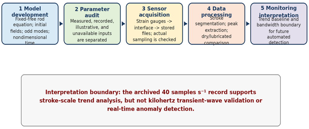
The analysis workflow to link between the theoretical model and the recorded sensor data is summarized in Figure 1, which also sets the boundary between stroke-scale monitoring and transient-wave measurement.
Figure 1. Auditable stroke-scale sensing and analysis workflow
2.1 Theoretical framework
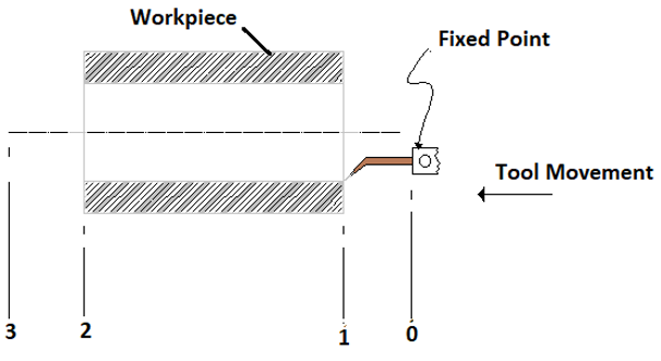
The shaping cycle has an active cutting stroke and an unloaded return stroke. A set of tool positions are used in the original kinematic description, which is shown in Figure 2. In modeling the exposed length of the tool is assumed to be a prismoidal rod of length L and area A, with Young's modulus E and density ρ. The clamped end is at x = 0 and the tool tip is at x = L. The model ignores damping and assumes small axial displacement, linear elasticity and constant material properties. It offers a clear structural starting point; it is not a simulation of the three-dimensional tool-contact problem or time-varying boundary conditions.
Figure 2. Schematic representation of the shaping stroke
Define u(x, t) to be axial displacement and F(x, t) to be the internal axial force. This idealization could be a longitudinal motion following to a given initial displacement or velocity field. It is not a claim that such a transient has been solved experimentally. Prior to claiming experimental validation, the expected modal time scale must be compared with the acquisition bandwidth.
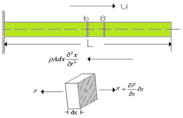
Axial force balance on a differential element gives (Figure 3).
$\frac{\partial F}{\partial x}=\rho A \frac{\partial^2 u}{\partial t^2}$ (1)
For a linear elastic rod, the axial force is
$F=A \sigma=E A \varepsilon=E A \frac{\partial u}{\partial x}$ (2)
$\frac{\partial^2 u}{\partial t^2}=a^2 \frac{\partial^2 u}{\partial x^2}, a=\sqrt{\frac{E}{\rho}}$ (3)
Figure 3. One-dimensional tool idealization and axial force balance
The symbol a denotes the longitudinal wave speed, not “stress velocity.” For a fixed-free rod, the natural frequencies depend on E, ρ, and the specimen-specific free length L. The archived record contains neither specimen-specific E, ρ, L, nor damping. Accordingly, Table 1 classifies model inputs as measured, recorded, illustrative, or unavailable; only the illustrative frequency scale is used for the bandwidth assessment.
Table 1. Model inputs, provenance, and role in the present analysis
|
Input or Quantity |
Value or Status |
Use and Provenance |
|
L |
Specimen-specific free length unavailable; 0.10–0.20 m used only for illustrative modal scale. |
Sets modal frequencies; not a measured specimen input. |
|
A |
Tool cross-section unavailable. |
Needed for force/stress conversion; it cancels out for a uniform rod. |
|
E |
210 GPa used for illustrative scale only; not measured for the specimen. |
Sets the longitudinal wave speed a. |
|
ρ |
8100 kg m⁻³ used for illustrative scale only; not measured for the specimen. |
Sets the longitudinal wave speed a. |
|
Damping |
Set to zero by model assumption; no damping record archived. |
Defines the undamped baseline; not a measured property. |
|
u(x, 0), ∂u/∂t(x, 0) |
Initial fields stated symbolically; numerical fields unavailable. |
Set modal coefficients and predicted history. |
|
Retained modes N and Δt |
Not archived. |
Control truncation and time integration; peak reproducibility cannot be independently checked. |
|
V₀ |
0.0042, 0.042, 0.147, 0.252 m s⁻¹; recorded command values. |
Speed comparison; reported in Section 3. |
|
ε₀a |
0.105 m s⁻¹; fixed in archived calculation; provenance unavailable. |
Normalizes MP; makes MP proportional to V₀ in this dataset. |
For sensitivity of the modal scale, a = √(E/ρ) and the first fixed–free modal frequency is f₁ = a/(4L). Thus, small relative changes follow δa/a ≈ 1/2(δE/E − δρ/ρ) and δf₁/f₁ ≈ δa/a − δL/L. A ±10% change in E alone changes a and f₁ by approximately ±5%, whereas a ±10% change in L changes f₁ by approximately $\mp$ 10%. These calculations describe modal-frequency sensitivity only. Because the retained-mode count, time step, and numerical initial fields are not archived, a corresponding sensitivity interval for the calculated peak strains cannot be reconstructed without inventing input data. For scale only, E = 210 GPa and ρ = 8100 kg m⁻³ give a ≈ 5.09 km s⁻¹; a free length of 0.10-0.20 m gives an illustrative first frequency of approximately 6.4-12.7 kHz, far above the 20 Hz Nyquist frequency of the stored record.
2.1.1 Fixed-free rod solution
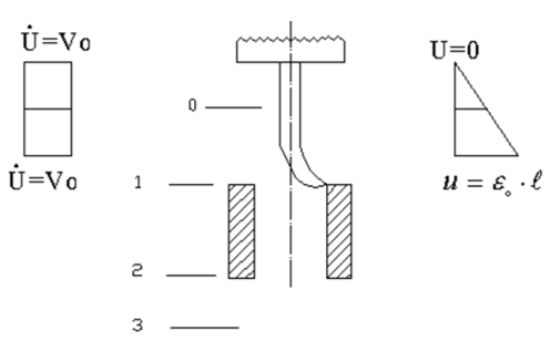
Separation of variables is introduced, see Figure 4, as:
$u(x, t)=X(x) T(t)$ (4)
Substitution into Eq. (3) yields the spatial and temporal equations
$X^{\prime \prime}+k^2 X=0, T^{\prime \prime}+(a k)^2 T=0$ (5)
$u(0, t)=0,\left.\frac{\partial u(x, t)}{\partial x}\right|_{x=L}=0$ (6)
The fixed–free boundary conditions admit only odd modes:
$\begin{gathered}k_n=\frac{(2 n-1) \pi}{2 L}, \omega_n=a k_n, f_n=\frac{(2 n-1) a}{4 L} \\ n=1,2,3, \ldots\end{gathered}$ (7)
The displacement is therefore
$u(x, t)=\sum_{n=1}^{\infty}\left[A_n \cos \left(\omega_n t\right)+B_n \sin \left(\omega_n t\right)\right] \sin \left(k_n x\right)$ (8)
The initial displacement and velocity fields must be stated explicitly:
$f(x)=u(x, 0), g(x)=\left.\frac{\partial u(x, t)}{\partial t}\right|_{t=0}$ (9)
From the orthogonality of the modes, the coefficients are:
$A_n=\frac{2}{L} \int_0^L f(x) \sin \left(k_n x\right) d x$ (10)
and
$B_n=\frac{2}{L \omega_n} \int_0^L g(x) \sin \left(k_n x\right) d x$ (11)
The spatial derivative gives the axial strain at a given point x:
$\begin{gathered}\varepsilon(x, t)=\frac{\partial u}{\partial x}=\sum_{n=1}^{\infty} k_n\left[A_n \cos \left(\omega_n t\right)+B_n \sin \left(\omega_n t\right)\right] \cos \left(k_n x\right)\end{gathered}$ (12)
$\tau=\frac{a t}{L}$ (13)
$M P=\frac{V_0}{\varepsilon_0 a}$ (14)
Figure 4. Definition of the reference displacement and velocity by kinematic idealization
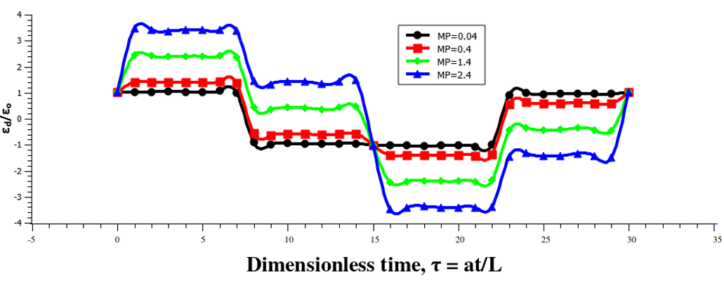
The old term “Mechanical Properties Variable” is changed to “dimensionless machining parameter” (MP), not because it is a property of the material, but to avoid any such implication. The commanded tool speed (V₀) given in Table 2, the reference strain (ε₀) for normalization, and the longitudinal wave speed (a) are used. It was determined that the product ε₀a = 0.105 ms⁻¹ was constant in the archived calculation, so that the four values of MP are proportional to V₀. The MP is only kept as a description parameter of the normality, not as a new predicting criterion or as an independent material variable, see Figure 5.
Figure 5. Legacy curves plotted against the new nondimensional time τ = a t/L; MP is the dimensionless machining parameter. The original count in retained mode, the original time step, the convergence study and the original fields were not saved
Table 2. Reported chemical composition of the high-speed steel (HSS) M2 cutting tool
|
C% |
Cr% |
Mo% |
W% |
V% |
Co% |
|
0.9 |
4.1 |
5 |
6 |
2 |
0.05 |
2.2 Experimental work
2.2.1 Tool and workpiece materials
The cutting tool was said to be HSS M2 and the workpiece was American Iron and Steel Institute (AISI) 1144 steel. Elemental compositions were measured for their and presented in Tables 2 and 3. The analyses were carried out in the General Company for Mechanical Industries, Babylon in a photoelectric Spectrometer. The test record was not archived with mechanical properties necessary for the prediction of modal response specific to the specimen, such as measured E, ρ, hardness, and damping.
Table 3. Reported chemical composition of the American Iron and Steel Institute (AISI) 1144 workpiece
|
C% |
Si% |
Mn% |
S% |
P% |
|
0.45 |
0.4 |
1.5 |
0.3 |
0.06 |
2.2.2 Experimental setup and procedure
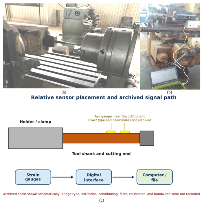
The experiments were carried out in Al-Musayyib Technical Institute in the workshops on a modified milling machine. The machine was set up to cut a reciprocating internal shaping cut in a cylindrical workpiece as displayed in Figure 6(a). The tool was attached to the tool holder and the work piece was latched on to the dividing head. Cutting depth was maintained at 1.5 mm, and the commanded speeds were 0.0042, 0.042, 0.147, and 0.252 ms⁻¹. The recorded arrangement represents manual/offline acquisition; no automatic closed-loop monitoring function was archived.
Figure 6. (a) Modified milling machine configured for the internal shaping operation; (b) instrumented tool, strain interface, and acquisition computer; (c) schematic of relative strain-gauge placement and the archived signal path; gauge specifications and exact locations were not recorded
The instrumented arrangement is depicted in Figure 6(b) and the signal path that is archived is summarized in a schematic in Figure 6(c). Two strain gauges were placed close to the cutting end and hooked up to a digital interface and computer. The relative placement is shown only in a schematic way as the archived report does not contain any information on machine model, tool dimensions, overhang, cross-section, rake/clearance/edge angle, workpiece dimensions and hardness, feed per stroke and stroke length, gauge model, resistance, gauge factor, orientation, exact coordinates, bridge type and excitation voltage, amplifier/filter bandwidth, calibration procedure, machine deceleration/reversal profile, or application rate or temperature of the lubricant. Such omissions do not allow independent reproduction in full, and are considered explicit restrictions and not filled in by assumed values. Table 4 reports the composition of the oil-based lubricant.
Table 4. Reported composition of the oil-based lubricant
|
Component |
Reported Function |
Volume Fraction |
|
Base oil |
Base fluid |
75% |
|
Emulsifying soap |
Emulsifier |
11% |
|
Carbolic acid (phenol) |
Biocide |
7% |
|
Sulfur-based additive (reported) |
Extreme-pressure additive |
7% |
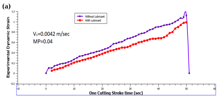
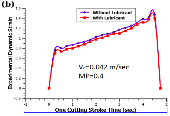
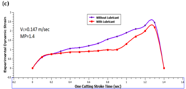
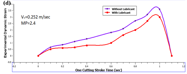
The acquisition hardware was described as having a nominal 120 Hz setting, whereas the exported data files contained 40 samples s⁻¹. The archived signal chain was strain gauges → digital interface → computer; the gauge frequency response, bridge type, excitation, amplifier, filter, anti-aliasing, and calibration records were not available. All plots and peak values are based on the stored 40 samples s⁻¹ series, whose Nyquist frequency is 20 Hz. This rate can describe a slowly varying signal over a complete cutting stroke when sufficient samples span the stroke, but it cannot resolve the calculated kilohertz longitudinal modes. It is therefore appropriate only for the stated stroke-scale, quasi-dynamic peak analysis, not for dynamic-system validation. The plotted histories describe strain variation over the complete cutting stroke. The terminal fall in Figure 7 marks the end of the recorded stroke, but it is not evidence of an instantaneous stop, ringing, wave reflection, or decay. For each condition, peak stroke-scale strain was defined as the maximum stored sample before the terminal fall. Only one archived peak value per speed and lubrication condition was available; replicate-level time histories and uncertainty records were not available.
In Figure 7, as the cutting proceeds, the measured strain increases gradually until the end, when a sudden drop occurs. There is no indication of resolvable post-stop oscillation or ringing in the records, and therefore the extracted maxima are interpreted as peak cutting-stroke strain rather than as strain produced specifically by an abrupt stop. The four model peaks have been compared with the dry and lubricated measurements in Table 5.
Table 5. Model and measured peak stroke-scale strain under dry and lubricated cutting; MP denotes the dimensionless machining parameter
|
Case |
MP |
Vc (ms⁻¹) |
εPeak, Model |
εPeak, Dry |
εPeak, Lubricated |
|
1 |
0.04 |
0.0042 |
0.0007 |
0.00084 |
0.0007 |
|
2 |
0.4 |
0.042 |
0.001 |
0.001 |
0.00098 |
|
3 |
1.4 |
0.147 |
0.00169 |
0.00172 |
0.00154 |
|
4 |
2.4 |
0.252 |
0.00238 |
0.00252 |
0.0021 |
To position the present baseline for process monitoring and intelligent manufacturing, Table 6 compares it with related studies cited in the manuscript. The processes, measured variables, and acquisition systems differ; therefore, numerical values are reported only for the present archived data, while the other rows summarize their reported variables and scope.
Table 6. Comparison with related machining, sensing, and lubrication studies; root mean square error (RMSE) denotes root mean square error and minimum quantity lubrication (MQL)
|
Study or Approach |
Model and Method |
Measured Variable and Principal Finding |
|
Present study |
Fixed–free rod baseline paired with archived strain-gauge records. |
Stroke-scale peak strain; four speed conditions; dry/model RMSE = 1.001 × 10⁻⁴ and descriptive trend agreement only. |
|
Malik and Gorana [1] |
Shaping-operation cutting-force experiment. |
Cutting force under shaping parameters; positions the present local-strain signal as complementary to force measurement. |
|
Storch and Zawada-Tomkiewicz [2] |
Analytical/distributed force treatment for constrained turning. |
Unit force around the tool nose; emphasizes load distribution rather than stroke-scale local strain. |
|
Zhu et al. [3] |
Longitudinal–torsional ultrasonic-drilling experiment. |
Tool-wear and machining-performance variables under high-frequency excitation; illustrates the bandwidth requirements of dynamic sensing. |
|
Pan et al. [4] |
Cutting-force observer for tool-deflection compensation. |
Force and tool deflection; demonstrates model-assisted process monitoring and compensation. |
|
Agrawal and Patil [27] |
MQL experiment on M2 steel. |
Cutting-fluid and machining-response variables; relevant to M2, but not the same lubricant protocol or archived signal chain. |
Dry peak values were also in an increasing trend like model values. The theoretical peaks ranged from 0.70 × 10⁻³ to 2.38 × 10⁻³, while the dry measurements ranged from 0.84 × 10⁻³ to 2.52 × 10⁻³. To make it clearer, root mean square error (RMSE), mean absolute error (MAE), mean absolute percentage error (MAPE) and R² are error or agreement descriptors. Prediction R² is a measure of residual error compared to observed variance while squared Pearson correlation (r²) is a measure of linear association. Both numbers are not good for transient-wave physics.
The absolute percentage errors of the four dry/model pairs were 20.0%, 0.0%, 1.78% and 5.88%. As a result, the RMSE, MAE, and MAPE are provided in Eqs. (15)–(17). No replicate measurements are taken and n = 4 peak pairs, so confidence intervals and inferential significance tests cannot be estimated. The metrics are sensitive to individual points and should therefore be used only as a descriptive indicator of the level of agreement in trends.
RMSE $=\sqrt{\frac{1}{N} \sum_{i=1}^N\left(\varepsilon_{\text {dry}, i}-\varepsilon_{\text {model}, i}\right)^2}=1.001 \times 10^{-4}$ (15)
$\begin{aligned} & \mathrm{MAE}=\frac{1}{N} \sum_{i=1}^N\left|\varepsilon_{\text {dry}, i}-\varepsilon_{\text {model}, i}\right|=7.75 \times 10^{-5} \\ & \mathrm{MAPE}=\frac{100}{N} \sum_{i=1}^N\left|\frac{\varepsilon_{\text {dry}, i}-\varepsilon_{\text {model}, i}}{\varepsilon_{\text {dry}, i}}\right|=6.91 \%\end{aligned}$ (16)
$\begin{gathered}R_{\mathrm{pred}}^2=1-\frac{\sum_{i=1}^N\left(y_{\mathrm{dry}, i}-\hat{y}_i\right)^2}{\sum_{i=1}^N\left(y_{\mathrm{dry}, i}-\bar{y}_{\mathrm{dry}}\right)^2}=0.9774 \\ r_{\text {Pearson }}^2=0.9913(N=4)\end{gathered}$ (17)
There was no evidence of an exponential dependence as claimed. For the four theoretical values, a linear fit gives εpeak = 0.0006946 + 0.006719Vc, with R² = 0.9993, whereas an exponential fit gives R² ≈ 0.964. This comparison is valid for a more-or-less linear correlation over the range of investigated speeds; other speeds and uncertainty estimates are needed to suggest a general constitutive relation.
The four increasing speeds gave recorded peak strains reductions of 16.7%, 2.0%, 10.5% and 16.7% under lubrication. This is consistent with the variation of the tool-chip friction or cutting load, but there is no force, temperature, friction, lubricant-flow or surface data in the archive. Others may include run-to-run variation, amount of application, thermal conditions, contact conditions, and signal conditioning. It is therefore reported as an observed association rather than a proven mechanism, as there is no evidence of the reduction through repeated trials, and so the statistical significance and uncertainty of the reduction cannot be determined.
MP is a product of the speed of the tools and the value of the reference product ε₀a and is therefore not a material property only. In this data set, MP is collinear with cutting speed as ε₀a was kept constant at 0.105 m s⁻¹, therefore this data set cannot be used to develop an independent material effect for MP. The parameter is not verified as a new impact criterion, whereas it is only kept as a compact nondimensional machining scale.
Theoretically, the model is an idealization of a linear-elastic one-dimensional ideal without any damping. In reality, the tools are three dimensional, the contact forces vary, the fixture is compliant, it is damped, and the boundary conditions are not modeled. No E, ρ, L, initial displacement and velocity fields, retained-mode count, time step or convergence results were archived. The difficulty of transient stress-wave validation is experimentally precluded by the 40 samples s⁻¹ files, unknown anti-aliasing and amplifier bandwidths, and the absence of a stop trigger and velocity and acceleration synchronization. These constraints also establish the minimum data necessary for an automated monitoring future implementation.
From a process-monitoring perspective, the workflow supports an offline baseline consisting of local strain acquisition, stroke-level peak extraction, and comparison with the analytical trend. The evidence supports only two findings: peak stroke-scale strain increased with commanded cutting speed, and the archived lubricated condition generally showed lower peaks than dry cutting. Real-time anomaly detection, vibration identification, wear assessment, fatigue prediction, surface-quality prediction, and tool-life improvement require synchronized high-bandwidth sensing, repeated trials, and direct outcome measurements and are not findings of this study.
A physically consistent fixed–free rod solution was presented for longitudinal displacement and strain, including odd modes, explicit initial fields, and nondimensional time τ = at/L. The illustrative modal calculation also shows that the expected longitudinal frequencies of an ordinary-sized HSS tool are far above the bandwidth of the archived strain record.
The experimental curves are considered quasi-dynamic, stroke-scale strain histories. Across four speeds, their dry peak values showed descriptive agreement with the model trend (RMSE = 1.001 × 10⁻⁴, MAE = 7.75 × 10⁻⁵, MAPE = 6.91%, and prediction R² = 0.9774). These four peak pairs are not proof of general model validity or transient stress-wave propagation.
Within the tested range, peak strain rose approximately linearly with commanded cutting speed. The archived peak values were 2.0-16.7% lower under lubrication, but the archive contains no replicate-level records; statistical significance and confidence intervals were therefore not estimated.
MP is a dimensionless machining parameter proportional to speed in the current dataset, so it has no demonstrated independent novelty or general predictive capability here. Claims about increased tool life, fatigue resistance, improved surface quality, damage reduction, or real-time monitoring remain beyond the measured evidence.
Future work should measure and report full tool and workpiece geometry and properties; characterize gauge and conditioning frequency response; sample at tens or hundreds of kilohertz as determined by the modal range; synchronize strain with an encoder, force channel, or accelerometer; and record a precisely triggered stop event. Replicated trials, uncertainty analysis, full time-history comparison, damping identification, and three-dimensional finite-element modeling are also required before automated transient monitoring or broader predictive claims can be evaluated.
[1] Malik, A.K., Gorana, V. (2015). Effects on cutting forces in shaping operation. European Journal of Advances in Engineering and Technology, 2(6): 20-23. https://ejaet.com/PDF/2-6/EJAET-2-6-20-23.pdf.
[2] Storch, B., Zawada-Tomkiewicz, A. (2012). Distribution of unit forces on the tool nose rounding in the case of constrained turning. International Journal of Machine Tools and Manufacture, 57: 1-9. https://doi.org/10.1016/j.ijmachtools.2012.01.011
[3] Zhu, Z.J., Geng, S.Y., Zhu, W.R., Guang, O.Y., Huang, Y.P. (2026). Evaluation of tool wear characteristics and machining performance during longitudinal-torsional ultrasonic vibration drilling of Al/Ti stacks. Micromachines, 17: 227. https://doi.org/10.3390/mi17020227
[4] Pan, Z.M., Wang, L.B., Fang, Q., Sun, Z.C., Qu, W.T. (2022). Study on tool deflection compensation method based on cutting force observer for orbital drilling of CFRP/Ti stacks. Journal of Manufacturing Processes, 75: 450-460. https://doi.org/10.1016/j.jmapro.2021.12.058
[5] Wang, Y.B., Pang, S.Q., Yan, P., et al. (2023). The effect of cutting fluid on high strain rate dynamic mechanical property and cutting force of ultra-high-strength steel. Journal of Materials Research and Technology, 25: 736-749. https://doi.org/10.1016/j.jmrt.2023.05.259
[6] Wang, Y., Wang, X.B., Liu, Z.B., et al. (2022). A plastic strain energy method exploration between machined surface integrity evolution and torsion fatigue behaviour of low-alloy medium-carbon steel. Chinese Journal of Aeronautics, 35(10): 412-429. https://doi.org/10.1016/j.cja.2021.11.003
[7] Shi, L.C., Wang, J., Dou, W.T., Yuan, J.G. (2024). Simulation on dynamic characteristics of TC4 cutting with crack defects. Journal of Measurement Science and Instrumentation, 15(3): 387-396. https://doi.org/10.62756/jmsi.1674-8042.2024040
[8] Huang, Z.K., Sun, W. (2021). Formation mechanism of adiabatic shear band during dynamic plastic deformation of titanium alloy. Materials Reports, 35(3): 3122-3128. https://doi.org/10.11896/cldb.19070111
[9] Pape, F., Poll, G., Ellersiek, L., Denkena, B., Liu, H.C. (2023). Tribological effects of metalworking fluids in cutting processes. Lubricants, 11(5): 224. https://doi.org/10.3390/lubricants11050224
[10] Pape, F., Liu, H.C., Ellersiek, L., Krödel, A., Denkena, B., Poll, G. (2022). Influence of metal working fluids in cutting processes. Defect and Diffusion Forum, 414: 51-57. https://doi.org/10.4028/p-dnly6l
[11] Hamzah, A.H., Al-Khafaji, H.M.H., Hussein, T.S. (2024). Optimizing aging time to maximize hardness and fatigue strength of Al–4 wt% Cu alloy. International Journal of Heat and Technology, 42(1): 297-302. https://doi.org/10.18280/ijht.420131
[12] Quintana, G., Ciurana, J. (2011). Chatter in machining processes: A review. International Journal of Machine Tools and Manufacture, 51(5): 363-376. https://doi.org/10.1016/j.ijmachtools.2011.01.001
[13] Siddhpura, M., Paurobally, R. (2012). A review of chatter vibration research in turning. International Journal of Machine Tools and Manufacture, 61: 27-47. https://doi.org/10.1016/j.ijmachtools.2012.05.007
[14] Munoa, J., Beudaert, X., Dombovari, Z., et al. (2016). Chatter suppression techniques in metal cutting. CIRP Annals, 65(2): 785-808. https://doi.org/10.1016/j.cirp.2016.06.004
[15] Li, Z.M., Song, Q.H., Jin, P.J., Liu, Z.Q., Wang, B., Ma, H.F. (2024). Chatter suppression techniques in milling processes: A state-of-the-art review. Chinese Journal of Aeronautics, 37(7): 1-23. https://doi.org/10.1016/j.cja.2023.10.001
[16] Jawahir, I.S., Brinksmeier, E., M’Saoubi, R., et al. (2011). Surface integrity in material removal processes: Recent advances. CIRP Annals, 60(2): 603-626. https://doi.org/10.1016/j.cirp.2011.05.002
[17] Novovic, D., Dewes, R.C., Aspinwall, D.K., Voice, W., Bowen, P. (2004). The effect of machined topography and integrity on fatigue life. International Journal of Machine Tools and Manufacture, 44(2-3): 125-134. https://doi.org/10.1016/j.ijmachtools.2003.10.018
[18] Liu, G.L., Huang, C.Z., Zhao, B., Wang, W., Sun, S.F. (2021). Effect of machined surface integrity on fatigue performance of metal workpiece: A review. Chinese Journal of Mechanical Engineering, 34: 118. https://doi.org/10.1186/s10033-021-00631-x
[19] Kolsky, H. (1949). An investigation of the mechanical properties of materials at very high rates of loading. Proceedings of the Physical Society. Section B, 62(11): 676-700. https://doi.org/10.1088/0370-1301/62/11/302
[20] Follansbee, P.S., Frantz, C. (1983). Wave propagation in the split Hopkinson pressure bar. Journal of Engineering Materials and Technology, 105(1): 61-66. https://doi.org/10.1115/1.3225620
[21] Shannon, C.E. (1949). Communication in the presence of noise. Proceedings of the IRE, 37(1): 10-21. https://doi.org/10.1109/JRPROC.1949.232969
[22] Davies, R.M. (1948). A critical study of the Hopkinson pressure bar. Philosophical Transactions of the Royal Society of London. Series A, Mathematical and Physical Sciences, 240(821): 375-457. https://doi.org/10.1098/rsta.1948.0001
[23] Lawal, S.A., Choudhury, I.A., Nukman, Y. (2012). Application of vegetable oil-based metalworking fluids in machining ferrous metals—A review. International Journal of Machine Tools and Manufacture, 52: 1-12. https://doi.org/10.1016/j.ijmachtools.2011.09.003
[24] Lawal, S.A., Choudhury, I.A., Nukman, Y. (2013). Developments in the formulation and application of vegetable oil-based metalworking fluids in turning process. International Journal of Advanced Manufacturing Technology, 67(5-8): 1765-1776. https://doi.org/10.1007/s00170-012-4607-0
[25] Debnath, S., Reddy, M.M., Yi, Q.S. (2014). Environmental friendly cutting fluids and cooling techniques in machining: A review. Journal of Cleaner Production, 83: 33-47. https://doi.org/10.1016/j.jclepro.2014.07.071
[26] Shashidhara, Y.M., Jayaram, S.R. (2010). Vegetable oils as a potential cutting fluid—An evolution. Tribology International, 43(5-6): 1073-1081. https://doi.org/10.1016/j.triboint.2009.12.065
[27] Agrawal, S.M., Patil, N.G. (2018). Experimental study of non-edible vegetable oil as a cutting fluid in machining of M2 steel using MQL. Procedia Manufacturing, 20: 207-212. https://doi.org/10.1016/j.promfg.2018.02.030
[28] Benedicto, E., Carou, D., Rubio, E.M. (2017). Technical, economic and environmental review of the lubrication/cooling systems used in machining processes. Procedia Engineering, 184: 99-116. https://doi.org/10.1016/j.proeng.2017.04.075
[29] Liao, Z., La Monaca, A., Murray, J., et al. (2021). Surface integrity in metal machining—Part I: Fundamentals of surface characteristics and formation mechanisms. International Journal of Machine Tools and Manufacture, 162: 103687. https://doi.org/10.1016/j.ijmachtools.2020.103687
[30] La Monaca, A., Murray, J.W., Liao, Z., et al. (2021). Surface integrity in metal machining—Part II: Functional performance. International Journal of Machine Tools and Manufacture, 164: 103718. https://doi.org/10.1016/j.ijmachtools.2021.103718