
Inam S. Naser | Ekhlas Falih Naser*
© 2026 The authors. This article is published by IIETA and is licensed under the CC BY 4.0 license (http://creativecommons.org/licenses/by/4.0/).
OPEN ACCESS
The method of creating a brief and concise synopsis of a longer video while preserving its main ideas and information is known as video abstraction. It is frequently used in computer science for intelligent video management, in academia for introducing published papers, and in the arts. Due to the proliferation of social media platforms, messaging applications, and portable video recording devices, videos are now widely shared and have become part of everyday life. However, anyone can edit videos due to the availability of many user-friendly applications. Videos that have been intentionally altered may spread false information and cause other negative consequences. This study aims to detect and eliminate interpolated video frames based on a Harris corner detector combined with histogram equalization and cosine similarity to produce an abstract video without visual artifacts or ghosting effects. The proposed methodology consists of two main stages. In the first stage, frames are extracted from the video, and the video frames are interpolated using the bicubic algorithm to determine the most precise interpolation. The fundamental concept of bicubic interpolation is to utilize a third-order polynomial to adapt to a surface between four corner points. The intensity values and the vertical, diagonal, and horizontal derivatives at each location of the four corners are required to calculate a bicubic interpolation. The second stage includes four steps. First, the video stream is split into a number of separate frames. These video frames are then resized to fixed dimensions of 256 × 256 pixels as part of the preprocessing process. Second, pixel intensities are mapped using histogram equalization, which extends the most common intensity values. Third, the features of each frame are extracted using a Harris corner detector, and the cosine similarity formula is then used to extract the interpolated frame in the fourth step. When studying color data for color blindness applications, cosine similarity is a useful tool that performs a mathematical comparison of Red Green Blue (RGB) space color vectors. From the empirical outcomes, it was noted that the precision was 94.15, recall was 90.33, and F1-score was 92.20 in the hammering video because a greater number of recurring features across frames were provided by the richer and more structured visual information found in the hammering frames, such as object boundaries, edges, and texture areas; thus, the evaluation results appeared high. This was followed by the hair-drying video, which contains less visual information and structure due to the relatively homogeneous background with limited texture in these frames, while the planets video obtained the lowest values because it contains large regions with a relatively homogeneous space background, limited texture, and fewer stable angle-like structures.
bicubic interpolation, cosine similarity, Harris corner detector, histogram equalization, video abstraction, video processing
In processing of video, such as conversion of frame rate, encoding of video, creating video with slow motion, interpolation of video frames is used to create a new frame between two successive frames [1]. However, a significant obstacle to the authenticity of the interpolated frames is the video content's complicated information, such as irregular object shapes, different motion patterns, occlusion problems, etc. [2]. An increasing number of researchers are using deep learning techniques to interpolate video frames as a result of deep learning's widespread development in computer vision. In order to forecast the intermediate, a popular technique in this field is the flow-based method, which warps the reference of frames' input relied on the flow of optical between the interpolation frame and the right and left reference frames [3].
Many academics have created models for interpolation of frames via utilizing end-to-end flow estimation, such as Deng et al. [4] and Sadiq et al. [5]. Nevertheless, the model is unable to forecast the precise flow information of optical flow between the frame's reference and the interpolated frame since these frames do not actually exist. Therefore, when the optical flow is inappropriate, low-quality images are produced. The author proposes a kernel-based approach that views interpolation of the pixel as the convolution of matching picture blocks in two frames of reference [6].
The kernel-based approach is more flexible than the flow-based approach. In order to approximate the spatially adaptive kernel of convolution, which combines estimation of synthesis and motion of pixels into just one process, it employs a deep convolutional neural network (CNN). This allows it to better handle difficult frame interpolation scenes. Nevertheless, the predicted frame's accuracy is constrained by the kernel size. In particular, the model can't manage huge objects that move if the size of the kernel is too small, yet it needs a lot of memory if the kernel size is set to a large value [7].
Despite lowering memory use, SepConv [8] is still unable to handle motion larger than the size of the predefined kernel. Currently, a number of researchers have created innovative algorithms to approximate the kernels of compensation and flow simultaneously with respect to the original frames of reference. These algorithms can tightly couple the approximation of motion and approximation of the networks of kernel in order to enhance the current frame using an overall model of the network. In one sense, by employing data-driven kernel coefficients, this approach can increase the interpolation accuracy in comparison to the flow-based approach, which depends on straightforward bilinear coefficients.
In contrast, the flow estimation model's anticipated optical flow first determines the approximate region of kernel's reference, which may significantly lower the size of kernel and achieve superior computing more efficient than the solitary kernel-based approach [9]. While these techniques have enhanced the interpolation of video frames, they all fail to take into account the uneven shape of the object and the unpredictable motion trajectory. As a result, the conventional convolution kernel shape is unable to adjust to different motions and objects. In this study, inspired by deformable convolution network (DCN) [10], it can be introduced to offset an adaptively reference pixels using the latent properties recovered via the network, such that the reference point's location becomes more useful.
Furthermore, according to DCNv2, not every pixel in the reference field contributes equally to the response of a target pixel, so we use both the coefficient of the kernel and the coefficient of bilinear to identify the variations within those contributions. Lastly, it can suggest a module of pixel synthesis to integrate the offset field, the interpolation kernel, and the optical flow in an adaptive manner [11].
The main contributions of this research are:
1. By rearranging pixel intensity values throughout the whole dynamic range, histogram equalization is a potent, parameter-free image processing method that improves global contrast. It works especially well for highlighting hidden details in both too-bright and gloomy areas and brightening underexposed photos.
2. Each frame's features were extracted using a Harris corner detector. The Harris corner detector's primary benefit is its invariance to changes in illumination, translation, and rotation. It reliably locates the same feature points even when an image is rotated, moved, or exposed to variable illumination because it uses image gradients rather than exact pixel values. It is very successful for feature extraction, stereo matching, and image stitching.
3. The cosine similarity formula was used to extract the interpolated frame. When studying color data for color blindness applications, cosine similarity is a very useful tool using a mathematical comparison of Red Green Blue (RGB) space color vectors.
The following are some of the approaches that the multimedia forensics community has sophisticated in current years to detect evidence of video frame-rate interpolation:
1. A motion-compensated detector of interpolation is proposed by Albrecht and Iske [12]. This strategy, in particular, depends on the assessment of the correlation that the interpolation filter introduced. This technique was first applied to address the issue of spatial resampling of images.
2. An additional study in the field of interpolation of video frame rates shows how to measure each encoded frame to identify interpolation footprints [13]. Additionally, video interpolation can be used to make a video faster (by cutting frames) or slower (by adding frames).
3. A CNN-based technique is used by the authors of this work [14] to differentiate between standard speed videos and sped-up videos. This work could result in the development of a new tool that is useful for identifying the frame-rate interpolation imprints found in videos. The goal of the effort is to be able to recognize a certain video as either original (untouched frame rate) or frame-rate interpolated. Therefore, a detector that can recognize frame-rate interpolation artifacts in a film can be suggested. The CNN processing stage and the Support Vector Machine (SVM) classifier comprise the detector. The goal is to retrieve a series of frames at a time from the film that is being examined. The batch of frames can be processed (using CNN) to create a feature vector that shows whether or not the segment has interpolation after being converted into numerous video domain versions. Ultimately, the SVM can be used to determine whether or not this feature vector has been used to interpolate the video.
4. In order to interpolate video frames, Al-Majidi and Mgharbel [15] proposed utilizing motion compensation and estimation in a neural network. It also recommended using an adaptive layer of warping to generate recent pixels that can approximate the compensation kernel and flow of optical at the same time. This extra warping layer was expected to have a close relationship with the motion estimation and kernel estimation networks.
5. Rukundo [6] introduced four weighting methods for digital picture interpolation procedures based on specific geometric features. Additionally, the normalized area was the metric used to express the weight of each form, especially when the total area exceeded one unit square. The four introduced schemes of weighting are founded on the minimum diameter of side-based (MD) within a regular tetragon, the hypotenuse-based radius (HR), the virtual pixel length-based height for the area of the triangle (AT), and the length of virtual pixel for the HR for the area of the circle (AC). The HR scheme-based non-traditional picture interpolation approach scored the highest at the reduced scale out of all those that were offered.
6. Pant et al. [16] presented a hybrid neural network called Learning Fusion Dual Stream CNN (LFDsN) that learns spatiotemporal representations from the residual and motion vector information in the compression domain in order to localize the deep interpolated frames (DIF). Initially, the motion regions' residual and motion vector are preserved via an intra-prediction constraint. Intrinsic tampering traces are further highlighted by subtracting the estimation of the residual or motion vector due to residual modulation or the MV refinement network.
7. Finally, discriminative representations are jointly trained from the enhancement traces using a dual-stream attention-based network. Extensive experimental results demonstrate that, when compared to conventional methods, the methodology can achieve state-of-the-art performance. Deep Interpolation of Video Frame Interpolation (VFI) video datasets produced by the most advanced deep VFI techniques have been assessed [17].
8. A key point-based key frame selection method is described in the study [18]. This method creates a worldwide key points collection founded on SIFT features derived from whole frames, and the frames that best cover the worldwide key points collection are chosen as key frames. To put it succinctly, the drawback of these kinds of key frame extraction techniques is that they might recover comparable key frames if the same information occurs in a film.
The proposed methodology went through two main stages: In the first stage, it involved extracting the frames from the video, and then the frames of video were interpolated by making use of the bicubic algorithm to determine the most precise interpolation. The basic idea behind bicubic interpolation is to employ a third-order polynomial function to fit a surface between four corner points.
To compute a bicubic interpolation, the intensity values and the horizontal, vertical, and diagonal derivates at the four corner points are required. The second stage included three steps. The video stream was split up into a number of separate frames in the first step. These video frames are then resized to fixed dimensions of 256 × 256 pixels as part of preprocessing. In the second stage, pixel intensities were mapped using an equalization of the histogram, which extended the most common values.
Significantly boosting global contrast, exposing hidden features in bright or dark areas, and functioning automatically without the need for manual parameter adjustment are its key benefits. In the third stage, each frame's features were extracted using a Harris corner detector and then the cosine similarity formula was used to extract the interpolated frame in the fourth stage. When studying color data for color blindness applications, cosine similarity is a very useful tool using a mathematical comparison of RGB space color vectors. Figure 1 illustrates the flowchart of the proposed methodology. The value of 0.7 was chosen as the limit for the cosine similarity threshold between the original frame and the interpolated frame from experiments on a large number of frames that were randomly tested and which showed that the cosine similarity values did not exceed 0.7.
Figure 1. A flowchart of the suggested system for extracting interpolated frames
3.1 Bicubic interpolation algorithm
A sophisticated image resampling technique called bicubic interpolation uses a weighted average of the 16 closest neighboring pixels (a 4 × 4 grid) to determine new pixel values. Compared to more straightforward techniques like nearest-neighbor or bilinear, it generates scaled images that are far smoother and more detailed [19]. The 16 nearby pixels of the unknown pixel P are included in the enlarged image's influence sphere. These 16 nearby pixels are then used to calculate P's color rate based on the pixels' distance from P. The bicubic interpolation algorithm is shown in Figure 2 [20].
Figure 2. Bicubic interpolation [20]
3.2 Histogram equalization
Equalization of Histogram is a sophisticated statistical method used in the processing of an image to enhance the creation of either light or dark images. g(x, y) is the final result of the processed image. The calculation of the transformation function sk for a given gray level rk can be illustrated in Eq. (1) [21]:
$g(x, y)=S_k=(L-1)^n=\sum_{i=0}^k p\left(r_j\right)$ (1)
where, P(rj) is the likelihood of the level of an intensity, rj in the original image, n is the total number of pixels in the image, and L is the total number of levels of intensity (often 256). HE utilizes four main stages to increase total image visibility and clarity [22]:
Stage_1. Calculate the Histogram: Determine how frequently each intensity level appears in the picture.
Stage_2. Determine the Cumulative Distribution Function (CDF) by adding the frequencies of each intensity level up to the present value.
Stage_3. Map and Normalize: Adjust the values of the CDF to the image's usable range (for example, 0 to 255 for an image with 8-bits).
Stage_4. Reassign the Pixels: utilize the newly modified values in place of the initial pixel intensities.
3.3 Harris corner detectors
When used in conjunction with other computer vision techniques, the Harris corner detector is among the most popular corner detectors for identifying features in photos and extracting corners. Because Harris's detector of corners directly considers the differential score of the corner for direction rather than employing shifting patches for each angle within 45 degrees, it proved to be more accurate than the prior one in distinguishing between edges and corners. Since then, it has been improved upon and utilized in several algorithms to get images ready for usage in subsequent processing steps [23].
The Harris corner algorithm's primary phases [24].
1. Estimation of gradient: The first stage is to calculate the input image's intensity gradients in the vertical (y) and horizontal (x) directions, which are represented as Iy and Ix, respectively. In order to lessen the impact of noise and small fluctuations, Sobel operators are used in conjunction with a Gaussian smoothing filter.
2. Gradient product calculation: The product and squared gradients Iy and Ix are calculated for each pixel in the image. In order to reduce processing time and improve computational efficiency, these operations are carried out in a vectorized way.
3. Gradient products for filtering of Gaussian: Next, a Gaussian filter is used to smooth the gradient products. In order to build the structural tensor for each pixel, this phase is essential for gathering data inside a local neighborhood.
4. Building the matrix of Harris: The matrix of Harris, also called the matrix of second-moment, is built at each location within a pixel using the smoothed gradient values. For computational efficiency, this matrix is constructed in a vectorized manner, capturing the intensity variation in the local region.
5. Calculating corner response: Function: Eq. (2) was utilized to determine the Harris detector's response for each pixel:
$R={det}(H)-k({trace}(H))^2$ (2)
where, (k) is the factor of a sensitivity that is usually configured to (0.04) based on empirical data from earlier. Researchers, the Harris matrix, the trace and determinant are denoted by trace (H) and det(H), respectively.
6. Suppression of non-maximum and selection of point of interest: The response map is subjected to non-maximum suppression in order to distinguish discrete corners [25]:
•The response of corner (R) is contrasted with a predetermined threshold for every pixel.
•The 3 × 3 pixel neighborhood is assessed.
•The chosen points' coordinates and matching gradient vectors are saved for later processing.
•A pixel is kept as a legitimate interest point if its (R) value is higher than the threshold and the local maximum in its vicinity.
3.4 Cosine similarity
By computing the cosine of their angle, cosine similarity determines how similar two non-zero vectors are to one another. In particular, it is widely utilized in search queries, recommendation systems, text analysis, and document comparison in data analysis and machine learning [26].
The similarity measure establishes the separation between each data object in a dataset based on its feature dimensions. Greater resemblance is indicated by a smaller distance, whilst lower similarity can be displayed via a bigger distance. Cosine similarity is a useful metric for assessing the degree of similarity between data objects, regardless of their size. Data objects within a dataset are handled as vectors in cosine similarity. Eq. (3) was utilized to find the cosine similarity between two vectors [27].
$C S(x, y)=\frac{x.y}{\|x\| \times\|y\|}$ (3)
where, the product (dot) of vectors "x" and "y" is represented by x.y, the magnitude (length) of the two vectors "x" and "y" equals ||x|| and ||y||, the two vectors 'x' and 'y' are the regular product of ||x|| × ||y||.
3.5 The proposed algorithm
The proposed algorithm is explained in Algorithm 1.
|
Algorithm1: Extracting Interpolated Frame |
|
Input: Database which contains Original and Interpolated frames Output: Brief representation for Interpolated Frames. Begin: Step 1: //Load the video, extract all original frames, and store them in a database called (R), extract all interpolated frames and store them in a database called (Q) Step 2: Build a database D from R and Q Step 3: For i=1 to F. counter // F= no. of Frames in a database D
// HF_frame[i] and HF_frame[i+1] refere to Harris features form frames at locations (i) and (i+1) respectively.
If HF_frame[i] < HF_frame[i+1] then Frame[i] is interpolated Else: Frame[i+1] is interpolated End If: End If End For END |
The empirical outcomes of the suggested methodology are examined and explained in this section. The C# programming language was used to implement the suggested solution. Twenty different kinds of movies from the Kaggle dataset [28] were utilized to assess the suggested approach. The videos in the dataset are in color. Each frame's dimensions were standardized to 256 × 256 pixels by the suggested method. Several steps are included in the suggested methodology:
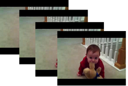
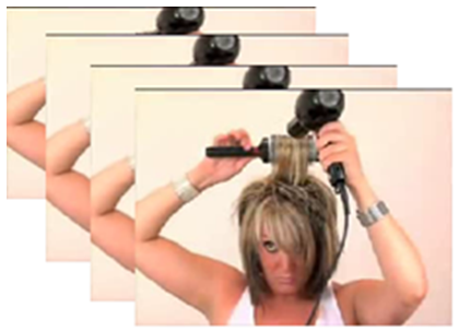
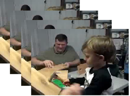
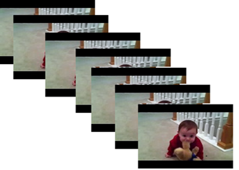
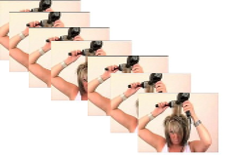
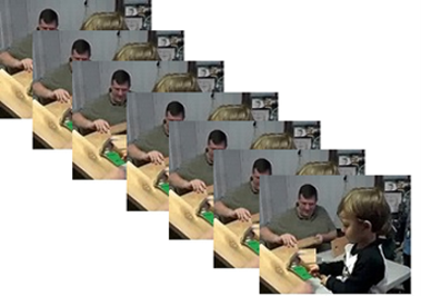
Step 1. All key frames were extracted after the movie was uploaded in the first step, as shown in Figure 3 for the Baby_1 video, Figure 4 for the hair drying video, and Figure 5 for the hammering video.
Step 2. As can be seen in Figure 6 for Baby_1 frames, Figure 7 for hair drying frames, and Figure 8 for hammering frames, the second step involved resizing every frame to a fixed size (256 × 256) and then using equalization of the histogram to enhance the frames.
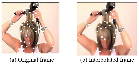
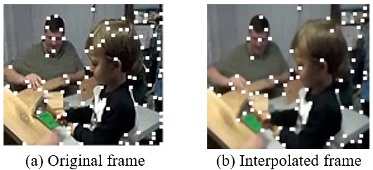
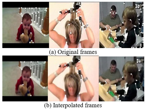
Step 3. Using the Harris corner detector, the sites of interest were identified in the third step. Figure 9 for Baby_1, Figure 10 for hair drying frames, and Figure 11 for hammering frames video provide an empirical representation of this step.
Figure 6. Samples of Baby_1 frames after histogram equalization
Figure 7. Samples of hair drying frames after histogram equalization
Figure 8. Samples of hammering frames after histogram equalization
Figure 9. Results of Harris corner detector for Baby_1
Figure 10. Results of Harris corner detector for hair drying
Figure 11. Results of Harris corner detector for hammering
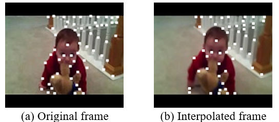
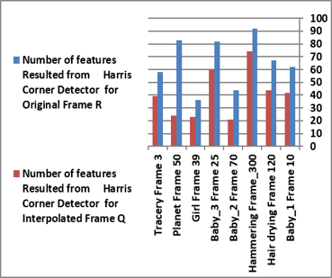
Step 4. The cosine similarity formula was used to extract the interpolated frame. Figure 12 illustrates the number of features that are extracted from the Harris corner detector for the samples of original frames and interpolated frames.
Figure 12. The number of features that are extracted from Harris corner detector for the samples of original frames and interpolated frames
Table 1 illustrates the results of the cosine similarity with the number of features resulting from the Harris corner detector for the samples of original and interpolated frames.
Table 1. The results of the cosine similarity
|
Frame Name |
Number of Features Resulted from Harris Corner Detector |
Cosine Similarity Between (R, Q) |
|
|
Original Frame R |
Interpolated Frame Q |
||
|
Baby_1 Frame 10 |
62 |
42 |
0.6507 |
|
Hair drying Frame 120 |
67 |
44 |
0.5510 |
|
Hammering Frame_300 |
92 |
74 |
0.5777 |
|
Baby_2 Frame 70 |
44 |
21 |
0.5024 |
|
Baby_3 Frame 25 |
82 |
60 |
0.6206 |
|
Girl Frame 39 |
36 |
23 |
0.5399 |
|
Planet Frame 50 |
83 |
24 |
0.1136 |
|
Tracery Frame 3 |
58 |
39 |
0.6092 |
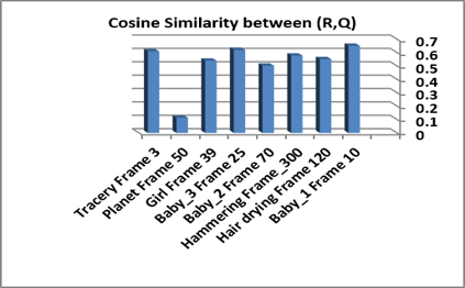
Figure 13 illustrates the values of cosine similarity for the same number of frames, but one frame was original and the other was interpolated.
Figure 13. The values of cosine similarity between the same frame numbers for original (R) and interpolated (Q)
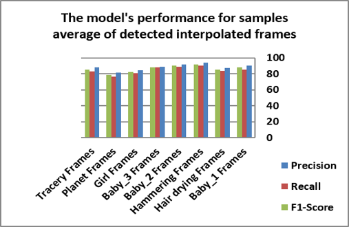
The precision, recall, and F1-score for extraction quality are determined using the suggested methods, as shown in Figure 14. The suggested method was used in Eq. (4) to calculate its precision. The recall of the suggested approach was calculated using Eq. (5) [29]. Additionally, the suggested method's F1-score was calculated via utilizing Eq. (6) [29]. The values of precision, recall, and F1-score are computed as shown in Table 2.
Figure 14. The average values of precision, recall and F1-score for detecting the sample average of interpolated frames
Table 2. The results of the precision, recall and F1-score for detecting the sample average of interpolated frames
|
Samples of Interpolated Frames |
Precision |
Recall |
F1-Score |
|
Baby_1 Frames |
90.72 |
85.55 |
88.06 |
|
Hair drying Frames |
87.3 |
84.17 |
85.71 |
|
Hammering Frames |
94.15 |
90.33 |
92.20 |
|
Baby_2 Frames |
91.82 |
88.96 |
90.37 |
|
Baby_3 Frames |
89.03 |
88.04 |
88.53 |
|
Girl Frames |
84.87 |
80.67 |
82.72 |
|
Planet Frames |
81.93 |
76.34 |
79.04 |
|
Tracery Frames |
88.04 |
82.90 |
85.39 |
Image scaling, which standardizes image sizes, is a resizing technique that reduces costs and execution time. Resizing an image by a factor is known as reducing its dimensions (256 and 256). Histogram equalization's main benefit is that, by uniformly spreading intensity values over the whole dynamic range, it greatly improves an image's overall contrast. This eliminates the need for manual parameter tweaking and reveals hidden subtleties in overexposed or underexposed areas.
$Precision =\frac{T P}{T P+F P}$ (4)
$Recall =\frac{T P}{T P+F N}$ (5)
$F 1- Score =\frac{{Precision} \times {Recall}}{{Precision}+ {Recall}} \times 2$ (6)
•The quantity of instances that are accurately classified as positive is referred to as True Positive ("TP").
•False Positive ("FP") refers to the quantity of instances that are incorrectly categorized as positive when the true status is negative.
•The quantity of instances that were accurately classified as negative is referred to as True Negative ("TN").
•The quantity of situations that are mistakenly classified as negative when the true state is positive is known as False Negative ("FN").
Additionally, it expands a small, constrained distribution of pixel values to make use of the entire spectrum of intensity.
In order to elicit features, the suggested methodology utilized a Harris corner detector. The Harris corner detector had great accuracy in locating informative feature locations, mathematical stability, and invariance to rotation and illumination. It effectively separates edges and flat areas from genuine corners without using intricate, moving picture patches. The Harris corner detector was also invariant to geometric transformations. It can recognize the same corners even when an image is translated (shifted) or rotated. The interpolated frame was taken out of the database using the cosine similarity measure. The primary benefit of cosine similarity is that it is not dependent on the magnitude of the vector. It precisely assesses how closely two things align in meaning or orientation, even if their overall sizes, lengths, or frequencies differ greatly, by measuring the angle between vectors rather than their distance. One of the main challenges in distinguishing between interpolated frames and genuine frames, for example, is the failure of using simple methods like the cosine similarity measure alone. Different brightness levels affect how the angle between the characteristic vectors is calculated, as Table 3 illustrates. This results in misleading values that make the original and interpolated frames more similar. Without the use of a Harris detector and histogram equalization, Table 3 displays the cosine similarity values for a random sample average of video frames to differentiate between original frames and interpolated frames found using cosine similarity alone.
Table 3. The cosine similarity values for the sample average of video frames
|
Video Name |
Cosine Similarity between (Original, Interpolated) |
|
Baby_1 |
0.9497 |
|
Hair drying |
0.8501 |
|
Hammering |
0.8767 |
|
Baby_2 |
0.9985 |
|
Baby_3 |
0.8389 |
|
Girl |
0.9196 |
|
Planet |
0.4126 |
|
Tracery |
0.9081 |
The most important challenge in the proposed methodology is to rely on points of interest, which are the corners, instead of relying on all pixels of the frame, in the process of detecting the interpolated frame. This reduces the time and complexity of the proposed algorithm and also utilizes a small storage space to implement the proposed methodology.
Comprehensive Benefits of Merging:
1. Discrimination Accuracy: The capacity to discern between photos that are authentic and those that have had new pixels added.
2. Durability: The capacity to withstand slight noise and changes in surrounding lighting.
3. Computational Efficiency: Relying on central, specified properties (angles and pitches) results in less data being processed compared to examining each pixel separately.
The proposed method fixed the threshold value at 1000 because, experimentally, this value yielded a suitable number of corners for all tested videos.
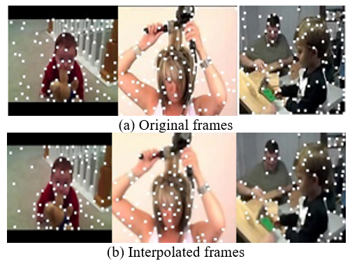
One of the main reasons for reducing angles in a Harris detector is threshold control. Raising the threshold value eliminates weak points and retains more accurate and consistent angles, as shown in Figure 15 when using a high threshold value of for example, 10000. In contrast, Figure 16 shows an increase in the number of corners because the detector detected even weak points when using a threshold value of, for example, 100.
Figure 15. Harris detector when using threshold = 10000
Figure 16. Harris detector when using threshold = 100
Table 4 illustrates the number of corners that result based on different thresholds.
Table 4. The results of the cosine similarity
|
Frame Name |
Number of Corners Resulted from Harris Corner Detector |
|||
|
Threshold = 100 |
Threshold = 10000 |
|||
|
Original Frame R |
Interpolated Frame Q |
Original Frame R |
Interpolated Frame Q |
|
|
Baby_1 Frame 10 |
100 |
87 |
31 |
12 |
|
Hair drying Frame 120 |
101 |
88 |
39 |
18 |
|
Hammering Frame_300 |
112 |
96 |
63 |
25 |
By avoiding visual abnormalities, ghosting, and motion blur, the primary benefit of removing interpolated frames in video abstraction is maintaining the structural integrity of the original source video. It guarantees that the abstracted movie or summary only uses real, unaltered camera footage. Removing synthetic, in-between frames offers a number of clear advantages:
1. Prevention of artifacts: When there is a lot of motion, synthesized frames frequently have obvious mistakes like deformed objects, twisted edges, or ghosting. Visual clarity is guaranteed when interpolation is dropped.
2. Accurate depiction: For abstraction of the video, the objective is to summarize a video's main points. By removing interpolation, the abstraction is guaranteed to use only authentic, unmodified content.
3. Decreased computational load: When the pipeline does not compute and render intermediate frames, the video abstraction process is substantially quicker and requires fewer resources.
The primary drawbacks of applying cosine similarity to match local feature descriptors derived from Harris corners include scale variance, geometric distortion, and cosine similarity's inability to take background noise and vector magnitude into account.
The following are the particular restrictions arranged according to their underlying causes:
1. Insufficient scale invariance scale
The issue: A fixed window size is used by the Harris detector to examine changes in intensity. The size of the corner in relation to the window varies whenever the camera zooms or the object's distance changes, which results in the detector failing.
Effect on Cosine Similarity: The gradient descriptors produced in the two images will not line up as a result of the corner structure shifting. Even with the identical physical feature, cosine similarity will result in low matching scores.
2. Sensitivity to changes in illumination and noise
The issue is that the Harris algorithm is very sensitive to changes in lighting and background noise because it directly depends on image derivatives.
Effect on Cosine Similarity: New gradient changes inside the descriptor window are introduced by noise. As a result, the descriptor vectors become "contaminated," drifting arbitrarily and producing inconsistent cosine similarity scores across frames.
How to get past these restrictions
Computer vision pipelines usually substitute the following for standalone cosine similarity and raw Harris patches in order to achieve strong feature matching:
1. Descriptors of Scale-invariant: Instead of using raw pixel patches, utilize ORB or SIFT descriptors.
2. By comparing the closest match to the second-closest match, the Distance Ratio of Nearest Neighbor (NNDR), which mathematically reduces spurious matches, is a better measure for distance than simple cosine or Euclidean matching.
This study focuses on identifying indications of interpolation for frame rate in video footage. As a result, a supervised learning classifier that can determine whether or not a video has undergone interpolation of frame rate can be made available. The proposed methodology makes utilize of the notion that different preprocessing methods can be used to improve the appearance of frame interpolation traces in the video being analyzed. After preprocessed videos were utilized to extract key features, the final extraction was done using cosine similarity. The approach has been validated by a number of experiments. For the research, a new dataset consisting of the original films and their associated interpolated versions at different frame rates can be made, starting with the UCF101 dataset. The proposed method relied on using the bicubic method to complete the interpolating process.
Because it yields far smoother and sharper results than simpler techniques (like bilinear or nearest-neighbor), bicubic interpolation is frequently utilized in digital images. It does this by using a 4 × 4 grid of 16 surrounding pixels, which is how programs like Adobe Photoshop accomplish this. By fitting a smooth, continuous curve (third-degree polynomial) across neighboring pixels, bicubic interpolation offers superior visual smoothness and eliminates the blocky or jagged "pixelation" that is present in lower-quality scaling techniques.
From Table 2, it was noted that the precision was 94.15, recall was 90.33, and F1-score was 92.20 in the hammering video because a greater number of recurring features across frames were provided by the richer and more structured visual information found in the hammering frames, such as boundaries of objects, edges, and areas of texture; thus, the evaluation results appeared high. After that came the hair-drying video, which contains less visual information and structure due to the relatively homogeneous background with limited texture in these frames, while the planets video got the lowest values because it contains large regions with a relatively homogeneous space background, limited texture, and fewer stable, angle-like structures.
The method proposed in this manuscript was not compared with CNN because it requires large data to perform the training process to achieve high accuracy, and because the detection method in this manuscript relies only on a few corner resulting from Harris. Therefore, the following is an illustration of the recommendations for more work:
1. To extract points of interest from video frames, I suggest utilizing the "Speeded-Up Robust Features" (SURF), "Oudemansiella raphanipies phenotype extractor" (ORP), or CNN techniques.
2. Video footage can be analyzed for information and events using recurrent neural networks and long short-term memory.
3. YOLO V11 can be employed to evoke interpolated frames in real-time situations.
This article is supported by the University of Technology/College of Computer Science, Baghdad/ Iraq.
[1] Abbas, A.R., Naser, E.F. (2025). Detecting interpolated video frames based on convolution neural networks. The Journal of Engineering Research, 22(2): 153-162. https://doi.org/10.53540/1726-6742.1317
[2] Briedis, K.M., Djelouah, A., Meyer, M., McGonigal, I., Gross, M., Schroers, C. (2021). Neural frame interpolation for rendered content. ACM Transactions on Graphics (TOG), 40(6): 1-13. https://doi.org/10.1145/3478513.3480553
[3] Daly, C., Ramsook, D., Kokaram, A. (2025). Efficient motion-based metrics for video frame interpolation. Applications of Digital Image Processing XLVIII, 13605: 315-326. https://doi.org/10.1117/12.3063574
[4] Deng, H.Q., Zhang, Z.X., Zou, S.H., Li, X.Y. (2023). Bi-directional frame interpolation for unsupervised video anomaly detection. In 2023 IEEE/CVF Winter Conference on Applications of Computer Vision (WACV), Waikoloa, HI, USA, pp. 2633-2642. https://doi.org/10.1109/WACV56688.2023.00266
[5] Sadiq, B.O., Bello-Salau, H., Abduraheem-Olaniyi, L., Muhammad, B., Olayinka Zakariyya, S. (2022). Towards enhancing keyframe extraction strategy for summarizing surveillance video: An implementation study. Journal of ICT Research and Applications, 16(2): 167-183. https://doi.org/10.5614/itbj.ict.res.appl.2022.16.2.5
[6] Rukundo, O. (2023). Normalized weighting schemes for image interpolation algorithms. Applied Science, 13(3): 1741. https://doi.org/10.3390/app13031741
[7] Rucka, M., Wojtczak, E., Zielińska, M. (2020). Interpolation methods in GPR tomographic imaging of linear and volume anomalies for cultural heritage diagnostics. Measurement, 154: 107494. https://doi.org/10.1016/j.measurement.2020.107494
[8] Jeczmionek, E., Kowalski, P.A. (2021). Flattening layer pruning in convolutional neural networks. Symmetry, 13(7): 1147. https://doi.org/10.3390/sym13071147
[9] Dubey, P., Dubey, P.K., Sharma, M., Changlani, S. (2022). Comparative performance analysis of various digital image edge detection techniques with hybrid edge detection technique which is developed by combining second order derivative techniques log and Canny. International Journal of Nonlinear Analysis and Applications, 13: 89-95. https://doi.org/10.22075/ijnaa.2022.6334
[10] Shi, Z.H., Liu, X.H., Shi, K.D., Dai, L.H., Chen, J. (2022). Video frame interpolation via generalized deformable convolution. IEEE Transactions on Multimedia, 24: 426-439. https://doi.org/10.1109/TMM.2021.3052419
[11] Tian, H., Gao1, P., Peng, X. (2022). Video frame interpolation based on deformable kernel region. In Thirty-First International Joint Conferences on Artificial Intelligence (IJCAI-22), pp. 1349-1355. https://doi.org/10.24963/ijcai.2022/188
[12] Albrecht, K., Iske, A. (2025). On the convergence of generalized kernel-based interpolation by greedy data selection algorithms. BIT Numerical Mathematics, 65: 5. https://doi.org/10.1007/s10543-024-01048-3
[13] Albrecht, K., Entzian, J., Iske, A. (2025). Product kernels are efficient and flexible tools for high-dimensional scattered interpolation. Advances in Computational Mathematics, 51: 14. https://doi.org/10.1007/s10444-025-10226-y
[14] Yoon, M., Nam, S.H., Yu, I.J., Ahn, W., Kwon, M.J., Lee, H.K. (2022). Frame-rate up-conversion detection based on convolutional neural network for learning spatiotemporal features. Forensic Science International, 340: 111442. https://doi.org/10.1016/j.forsciint.2022.111442
[15] Al-Majidi, H.S., Mgharbel, A. (2023). Development of a sequential CNN model with three hidden layers for diabetes prediction. Journal of Basrah Researches (Sciences), 49(2): 171-184. https://doi.org/10.56714/bjrs.49.2.14
[16] Pant, Y., Shah, G., Ojha, R., Thapa, R., Bhatta, B. (2023). Comparison of CNN architecture of image classification using CIFAR10 datasets. International Journal on Engineering Technology, 1(1): 37-52. https://doi.org/10.3126/injet.v1i1.60898
[17] Kulkarni, A.D. (2023). Multispectral image analysis using convolution neural networks. International Journal of Advanced Computer Science and Applications, 14(10): 13-19. https://doi.org/10.14569/IJACSA.2023.0141002
[18] Hasan, S.A., Hadi, G.M. (2024). Review about SIFT and local feature extraction in content based image retrieval. In 5th International Conference on Communication Engineering and Computer Science (CIC-COCOS’24), pp. 317-323. http://doi.org/10.24086/cocos2024/paper.1533
[19] Bambang, K., Ahmat, A. (2021). Analysis of medical image resizing using bicubic interpolation algorithm. Jurnal Ilmu Komputer, 14(1): 20-29. https://doi.org/10.24843/jik.2021.v14.i01.p03
[20] Abbas, A.R., Naser, E.F. (2025). Comparison between interpolation methods to determine the best method for video frames interpolation. AIP Conference Proceedings, 3282: 030007. https://doi.org/10.1063/5.0269934
[21] Goni, I., Malgwi, Y.M., Ahmadu, A.S. (2023). Satellite image enhancement using histogram equalization. Electrical Science & Engineering, 5(1): 9-20. https://doi.org/10.30564/ese.v5i1.5234
[22] Wu, M.Z., Zhong, Q.Y. (2024). Image enhancement algorithm combining histogram equalization and bilateral filtering. Systems and Soft Computing, 6: 200169. https://doi.org/10.1016/j.sasc.2024.200169
[23] Al-Jaberi, A.S., Rahman, S.F., Raheem, I.F. (2025). Integrating Harris corner detector and SIFT descriptor for high-accuracy feature matching in image processing. Journal of Al-Qadisiyah for Computer Science and Mathematics, 17(3): 179-190. https://doi.org/10.29304/jqcsm.2025.17.32455
[24] Sharma, S.K., Jain, K., Shukla, A.K. (2023). A comparative analysis of feature detectors and descriptors for image stitching. Applied Sciences, 13(10): 6015. https://doi.org/10.3390/app13106015
[25] Yildirim, M. (2024). Content-based image retrieval and image classification system for early prediction of bladder cancer. Diagnostics, 14(23): 2637. https://doi.org/10.3390/diagnostics14232637
[26] Steck, H., Ekanadham, C., Kallus, N. (2024). Is cosine-similarity of embeddings really about similarity? In WWW '24: Companion Proceedings of the ACM Web Conference 2024, Singapore, pp. 887-890. https://doi.org/10.1145/3589335.3651526
[27] Pevogam. (2020). UCF101 videos. Kaggle. https://www.kaggle.com/datasets/pevogam/ucf101.
[28] Naser, E.F. (2026). Video summarization based on the difference in statistical histograms of fuzzy clustering features. Baghdad Science Journal, 23(4): 1255-1269. https://doi.org/10.21123/2411-7986.5264
[29] Al-Abbasi, M., Naser, E.F., Kareem, T.A. (2026). Real-time fire and smoke detection and classification of video frames in smart cities based on You Only Look Once version 10 model. Journal Européen des Systèmes Automatisés, 59(5): 1195-1206. https://doi.org/10.18280/jesa.590502