
Tarek Bouguerra* | Laid Zarour | Aissa Bouzid
© 2026 The authors. This article is published by IIETA and is licensed under the CC BY 4.0 license (http://creativecommons.org/licenses/by/4.0/).
OPEN ACCESS
This manuscript introduces a backstepping-based nonlinear control strategy tailored for the vector-controlled induction motor (IM) drive of a standalone photovoltaic water pumping system (SPVWPS). Utilizing a multi-scalar formulation, the highly coupled induction machine model is decomposed into decoupled electromagnetic and mechanical subsystems, significantly streamlining the control synthesis and boosting dynamic responsiveness. The physical architecture incorporates a centrifugal pump load driven by an IM, which is energized by a standalone photovoltaic (PV) array paired with a lead–acid battery energy storage system. The proposed framework concurrently guarantees a seamless, resilient power supply under volatile atmospheric conditions and maximizes PV energy harvesting. Power extraction is governed by an enhanced variable-step-size (VSS) perturb and observe (P&O) maximum power point tracking (MPPT) technique with a backstepping controller, effectively mitigating steady-state oscillations by approximately 4 W while accelerating transient convergence time to 0.01s. Concurrently, an energy management strategy orchestrates bidirectional power flow to store excess solar energy and bridge generation deficits. MATLAB/Simulink simulations corroborate the superior performance of the integrated control framework based on the backstepping approach compared with traditional control paradigms using a Proportional-Integral (PI) regulator. Specifically, the proposed framework reduces the motor speed settling time from 0.7 s to 0.38 s, demonstrating improvements in response time and overall energy efficiency.
standalone photovoltaic water pumping system, maximum power point tracking, backstepping controller, multi-scalar model, induction motor, DC bus, battery storage
The global transition toward sustainable energy paradigms has accelerated the deployment of decentralized photovoltaic (PV) generation, particularly in regions lacking centralized electrical grids [1]. Among various localized applications, solar-powered water pumping systems have emerged as an economically viable solution for agricultural irrigation and municipal water supply in remote regions [2]. Despite their environmental advantages, the integration of PV-driven systems introduces significant operational complexities. The electrical output characteristics of PV arrays are inherently nonlinear and highly sensitive to stochastic atmospheric fluctuations, such as variations in solar irradiance and ambient temperature [3, 4]. To mitigate these fluctuations and guarantee optimal energy extraction, maximum power point tracking (MPPT) algorithms are indispensable components in modern PV architectures [5].
The perturb and observe (P&O) algorithm remains a widely adopted benchmark in commercial applications due to its computational simplicity and ease of hardware implementation. However, conventional fixed-step-size P&O techniques are prone to severe steady-state power oscillations around the maximum power point (MPP) and exhibit a notable trade-off between tracking speed and steady-state efficiency [6]. Numerous investigations indicate that adopting a variable-step-size (VSS) approach can partially alleviate these limitations by dynamically adjusting the perturbation increment to accelerate transient tracking and attenuate steady-state ripples [6, 7]. Nonetheless, because power electronic converters and PV sources exhibit highly nonlinear coupled dynamics, MPPT control fundamentally represents a complex nonlinear regulation problem. Consequently, advanced nonlinear control frameworks offer superior stability and dynamic efficiency compared to classical linear controllers [8].
Among these nonlinear strategies, backstepping control has emerged as a powerful recursive design methodology [8]. For instance, a hybrid two-loop backstepping controller was proposed in this study [9] for standalone PV applications, utilizing a regression plane for real-time MPP estimation. While conceptually sound, this framework suffered from substantial steady-state tracking errors and sluggish transient response. Although subsequent modifications managed to minimize the steady-state error [10], the system still exhibited pronounced overshoot and undershoot during rapid environmental transients.
Furthermore, a critical vulnerability of standalone PV systems is the intermittent nature of solar irradiance, which severely compromises the reliability of continuous water delivery [11]. To address this energy deficit, the integration of auxiliary electrochemical energy storage units—such as lead–acid battery banks—is crucial [12]. These storage systems serve a dual purpose: capturing surplus generation during peak irradiance intervals and supplementing the power demand during deficit periods or complete solar absence [13]. Such hybrid topologies substantially bolster the localized DC bus stability and elevate the overall operational reliability of the pumping infrastructure [13, 14].
Regarding the electromechanical drive subsystem, induction motors (IMs) are preferentially utilized in solar pumping systems due to their ruggedness, brushless construction, and minimal maintenance requirements [14]. However, the mathematical model of an IM is multi-variable, highly coupled, and intrinsically nonlinear, presenting significant control challenges [15]. Alternating current (AC) motor control strategies are generally classified into scalar and vector control methods. Although scalar control (V/f) is straightforward, its dynamic performance is inadequate for demanding applications [16]. Conversely, field-oriented vector control (FOC) achieves high dynamic precision by decoupling the rotor flux and electromagnetic torque via feedback loop linearization [17]. However, parametric variations and mechanical nonlinearities necessitate the application of nonlinear control laws to maintain high precision under both steady-state and dynamic load changes [18].
To handle these structural complexities, various nonlinear techniques—including input-output decoupling and feedback linearization—have been extensively researched [19]. Notably, the multi-scalar model-based control framework, introduced by Krzemiński [20], simplifies IM dynamics by transforming the complex machine equations into two fully decoupled linear subsystems representing the electromagnetic and mechanical states. By synthesizing backstepping control—which systematically constructs stable control laws utilizing Lyapunov stability criteria—with the multi-scalar formulation, it is possible to achieve tracking performance and parameter robustness while reducing mathematical complexity [21].
To address the gaps identified in previous literature, this paper presents the design, control, and implementation of a standalone PV water pumping system integrated with a battery energy storage system. The core contributions of this work are summarized as follows:
1. An enhanced VSS-P&O algorithm is integrated with a backstepping MPPT controller to drive a DC/DC boost converter, ensuring rapid MPP convergence within 0.01s and minimizing steady-state oscillations to less than 1 W.
2. A nonlinear backstepping controller is synthesized based on a decoupled multi-scalar IM formulation to regulate a centrifugal pump load mechanical speed, ensuring high dynamic tracking and decoupling performance under severe operating conditions.
3. A bidirectional DC/DC buck-boost converter is governed by a dedicated energy management strategy to actively stabilize the DC bus voltage at 515 V and optimize battery state-of-charge (SoC) profiles during surplus and deficit generation states.
The remainder of this manuscript is organized as follows: Section 2 describes the comprehensive physical architecture of the system and power stage configuration. Section 3 presents the mathematical modelling of the standalone PV-battery pumping system and provides a detailed formulation for each constituent component, including the multi-scalar transformation of the IM. Section 4 details the systematic synthesis of the proposed control law based on the backstepping approach. Section 5 delineates the operational modes of the energy management system and discusses the high-fidelity simulation results obtained via MATLAB/Simulink. Finally, Section 6 concludes the paper with a summary of the core findings and their practical engineering implications.
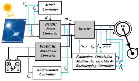
The standalone photovoltaic water pumping system (SPVWPS) under investigation features a two-stage energy conversion topology configured to maximize power extraction, regulate intermediate energy storage, and ensure high-precision electromechanical control. The comprehensive schematic architecture of the integrated system is illustrated in Figure 1.
Figure 1. Proposed system configuration
In the following sections three and four, respectively, the detailed modelling of each sub-system and the control design are provided. The primary power stage comprises a PV array connected to a high-efficiency DC/DC boost converter. This converter serves as the main impedance-matching interface, dynamically manipulating its switching duty cycle via an advanced MPPT algorithm to continuously harvest peak power under stochastically varying atmospheric conditions [5, 6]. The output of the boost converter is tied directly to a shared DC bus. To mitigate the structural intermittency of solar irradiance, a secondary power stage comprising a bidirectional DC/DC buck-boost converter interfaces a lead–acid battery storage bank with the DC bus, serving as a bidirectional power buffer [13].
The stabilized DC bus feeds a three-phase voltage source inverter (VSI), which performs DC-to-AC power conversion utilizing sinusoidal pulse-width modulation (SPWM) technique. The synthesized AC voltage is subsequently applied to the stator terminals of a three-phase IM, which is mechanically coupled to a centrifugal pump assembly designed for deep-well fluid extraction [14].
To establish a rigorous framework for the synthesis of the advanced nonlinear control and energy management strategies, a precise mathematical description of the standalone multi-source system is required. The integrated configuration under study consists of a PV array, a lead–acid battery storage unit, a bidirectional DC/DC converter, a DC/DC boost converter, a three-phase VSI, and an IM mechanically coupled to a centrifugal pump.
3.1 Photovoltaic generator modelling
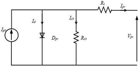
The PV generator converts solar irradiance directly into electrical energy. Utilizing the standard single-diode equivalent circuit model, which balances computational tractability and physical accuracy, the output current $I_{p v}$ of a PV module is governed by the following transcendental relationship:
$\begin{aligned} I_{p v}= & n_p I_{p h}-n_p I_o\left[\exp \left(\frac{q\left(V_{p v}+\frac{n_s}{n_p} R_S I_{p v}\right)}{n_s A K T}\right)-1\right] -\left(\frac{V_{p v}+\frac{n_s}{n_p} R_S I_{p v}}{\frac{n_s}{n_p} R_{s h}}\right)\end{aligned}$ (1)
where, $V_{p v}$ is the module voltage, $I_{p v}, I_{p h}, I_o$ are the module, photocurrent and the saturation current, $R_s, R_{s h}$ are the equivalent series and shunt resistance, respectively, $T$ is the temperature in Kelvin, $A$ is the ideality factor, $q$ is the electron charge, $k$ is the Boltzmann constant, $n_s$ and $n_p$ are the number of modules associated in series and parallel [3].
This mathematical relationship demonstrates the sharp nonlinear dependency of the MPP on erratic atmospheric variations, reinforcing the necessity of an MPPT controller.
The solar cell equivalent circuit is highlighted in Figure 2.
Figure 2. Equivalent circuit of a real solar cell
3.2 DC/DC boost converter dynamics and parametric design
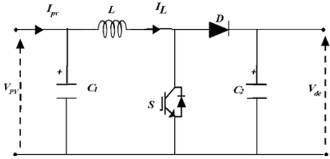
To efficiently interface the low-voltage PV array with the high-voltage shared DC bus, a step-up DC/DC boost converter is utilized as the primary impedance-matching topology (as shown in Figure 3). By actively manipulating the switching duty cycle, this converter tracks the MPP despite stochastic environmental fluctuations.
Assuming an ideal, lossless converter configuration, the state-space average mathematical model can be established to characterize the relationship between the input PV generation variables and the intermediate DC bus parameters. The steady-state voltage and current transformations are governed by the continuous conduction mode duty ratio d according to the following expressions:
$V_{d c}=\frac{V_{p v}}{1-d}$ (2)
$I_{d c}=(1-d) I_{p v}$ (3)
where, $V_{p v}$ and $I_{p v}$ denote the output voltage and current generated by the PV array, respectively, while $V_{d c}$ and $I_{d c}$ represent the voltage and current delivered to the shared DC link. The term $(1-d)$ signifies the continuous switching modulation index. To ensure low-ripple operation and maintain continuous conduction under peak load conditions, the physical energy storage elements-specifically the main boost inductor $L$ and the filtering capacitors-must be rigorously sized. The minimum input decoupling capacitance $C_1$, the output DC-bus filtering capacitance $C_2$, and the boost inductance $L$ are derived using the maximum allowable ripple thresholds via the following expressions (with the complete design parameters specified in Table 1).
Figure 3. The equivalent circuit of the boost converter
$L=d \frac{V_{p v}}{f \Delta I_L}$ (4)
$C_1=\frac{\Delta I_L}{8 f \Delta V_{p v}}$ (5)
$C_2=d \frac{I_{d c}}{f \Delta V_{d c}}$ (6)
where, $f$ designates the high-frequency pulse-width modulation switching frequency, $\Delta I_L$ is the peak-to-peak inductor current ripple, $\Delta V_{p v}$ represents the permitted input voltage ripple across the PV terminals, and $\Delta V_{d c}$ defines the maximum tolerable voltage ripple constraint imposed on the intermediate DC link. These computed parameters guarantee structural stability and minimize harmonic injection into the subsequent multi-scalar controlled IM drive loop.
Table 1. Boost parameters
|
L |
3 mH |
|
C1 |
600 µF |
|
C2 |
600 µF |
|
Switching frequency (f) |
20 kHz |
|
DC bus voltage (Vdc) |
515 V |
3.3 Mathematical modelling of the three-phase voltage source inverter
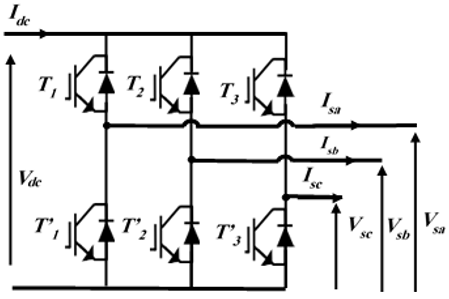
To drive the downstream three-phase IM utilizing the intermediate energy buffer, a two-level three-phase VSI is employed as the primary power stage interface. The schematic topology and equivalent circuit configuration of this three-phase bridge inverter are shown in Figure 4. The system incorporates six insulated-gate bipolar transistors (IGBTs) with anti-parallel freewheeling diodes, arranged into three distinct phase legs.
To prevent catastrophic short-circuits across the intermediate DC-link capacitor, the switching devices within each leg are modulated in a complementary fashion. Consequently, the instantaneous operational status of each inverter leg can be mathematically formalized by defining a discrete switching function $F_i(i \in\{1,2,3\}$, corresponding to inverter phases a, b, and c) as follows:
$F_i=\left\{\begin{array}{l}0, \text { if } T_i \text { is closed and } \, T_i^{\prime} \text { is open} . \\ 1, \text { if } T_i \text { is open and } \, T_i^{\prime} \text { is closed}\end{array}\right.$ (7)
Figure 4. Equivalent circuit of three-phase inverter
By evaluating the status of the upper switching states relative to the intermediate DC bus voltage ($V_{d c}$), the synthesized line-to-line stator voltages ($V_{a b}, V_{b c}, V_{c a}$) can be expressed in terms of these discrete switching vectors:
$\begin{aligned} & V_{a b}=V_{d c}\left(F_1-F_2\right) \\ & V_{b c}=V_{d c}\left(F_2-F_3\right) \\ & V_{c a}=V_{d c}\left(F_3-F_1\right)\end{aligned}$ (8)
Assuming a perfectly balanced three-phase motor configuration, the corresponding local phase-to-neutral terminal voltages $\left(V_a, V_b, V_c\right)$ are derived by transforming the line-to-line variables into the star-point reference framework:
$\begin{aligned} & V_a=V_{d c}\left(+2 F_1-F_2-F_3\right) / 3 \\ & V_b=V_{d c}\left(-F_1+2 F_2-F_3\right) / 3 \\ & V_c=V_{d c}\left(-F_1-F_2+2 F_3\right) / 3\end{aligned}$ (9)
Furthermore, by applying the principle of instantaneous power conservation across the input and output boundaries of the VSI, the total current drawn from the intermediate DC link $\left(I_{d c}\right)$ is mapped as a scalar product of the individual switching states and the respective alternating stator phase currents ($I_{s a}$, $\left.I_{s b}, I_{s c}\right):$
$I_{d c}=F_1 I_{s a}+F_2 I_{s b}+F_3 I_{s c}$ (10)
This comprehensive mathematical formulation yields the fundamental AC voltage profiles necessary to execute the non-linear multi-scalar backstepping speed control laws developed in Section 4.
3.4 Multi-scalar induction motor model
3.4.1 Classical (d-q) synchronous frame mathematical model
To establish the basis for the multi-scalar transformation, the fundamental continuous-time dynamics of a three-phase IM are initially formulated in a generic (d-q) synchronous reference frame rotating at an arbitrary primary angular frequency $\omega_s$ [15]. By choosing the stator currents $\left(i_{s d}, i_{s q}\right)$ and the rotor flux linkages ($\phi_{r d}, \phi_{r q}$) as the core state variables, the non-linear, cross-coupled state-space representation is governed by the following differential equations [15, 20]:
$\frac{d \phi_{r d}}{d t}=-\frac{R_r}{L_r} \phi_{r d}+R_r \frac{L_m}{L_r} i_{s d}+\left(\omega_s-\omega_m\right) \phi_{r q}$ (11)
$\frac{d \phi_{r q}}{d t}=-\frac{R_r}{L_r} \phi_{r q}+R_r \frac{L_m}{L_r} i_{s q}-\left(\omega_s-\omega_m\right) \phi_{r d}$ (12)
$\frac{d i_{s d}}{d t}=-\frac{1}{T_d} i_{s d}+\frac{R_r L_m}{L_r w_\delta} \phi_{r d}+\omega_s i_{s q}+\frac{L_m}{w_\delta} \omega_m \phi_{r q}+\frac{L_r}{w_\delta} u_{s d}$ (13)
$\frac{d i_{s q}}{d t}=-\frac{1}{T_d} i_{s q}+\frac{R_r L_m}{L_r w_\delta} \phi_{r q}-\omega_s i_{s d}-\frac{L_m}{w_\delta} \omega_m \phi_{r d}+\frac{L_r}{w_\delta} u_{s q}$ (14)
$\frac{d \omega_m}{d t}=\frac{L_m p}{J L_r}\left(-\phi_{r q} i_{s d}+\phi_{r d} i_{s q}\right)-\frac{p}{J} T l$ (15)
Such as, $\frac{1}{T_d}=\frac{L_r^2 R_s+L_m^2 R_r}{L_r w_\delta}$ and $w_\delta=L_s L_r-L_m^2$.
In this convention, $u_{s d}, u_{s q}$ designate the stator voltage inputs, $i_{s d}, i_{s q}$ denote the stator current space vector components, $\phi_{r d}, \phi_{r q}$ represent the rotor flux linkages, and $\omega_m$ signifies the mechanical rotor speed. The fixed machine parameters consist of the stator and rotor self-inductances ($L_s, L_r$), the mutual inductance ($L_m$), and the corresponding winding operational resistances ($R_s, R_r$). The mechanical parameters are represented by the external load torque $(T l)$, the comprehensive rotor moment of inertia $(J)$, and the number of pole pairs $(p)$.
3.4.2 Multi-scalar variable transformation definition
The structural non-linearities and strong electromagnetic cross-coupling evident in Eqs. (11)–(15) present severe challenges for high-performance linear control synthesis. To bypass these tracking limitations, a multi-scalar transformation framework is introduced. This framework converts the coordinate-dependent variables into four state variables that represent the scalar relationships between the flux and current vectors [22]:
$x_{11}=\omega_m$ (16)
$x_{12}=\phi_{r d} i_{s q}-\phi_{r q} i_{s d}$ (17)
$x_{21}=\phi_{r d}^2+\phi_{r d}^2$ (18)
$x_{22}=\phi_{r d} i_{s d}+\phi_{r q} i_{s q}$ (19)
The newly derived state vector possesses clear physical implications crucial for control loop partitioning:
$x_{11}$ maps the structural mechanical speed tracking trajectory directly.
$x_{12}$ represents the vector cross product between the rotor flux and stator current, which is directly proportional to the electromagnetic torque generation.
$x_{21}$ defines the absolute square of the rotor flux magnitude, tracking the magnetization state of the machine core.
$x_{22}$ expresses the vector dot product of the flux and current, which represents the reactive energy transition inside the stator-rotor coupling air gap.
3.4.3 Stator current space vector orientation
To achieve a completely decoupled structural format, the reference framework is aligned directly with the stator current space vector, forcing its quadrature component identically to zero $\left(i_{s q}=0\right)$. Furthermore, incorporating a first-order lag filter with an equivalent time constant $T_d$ within the stator current command loop yields a simplified set of orientation system dynamics:
$\frac{d i_{s d}}{d t}=\frac{1}{T_d}\left(i_{s d}-I_s^*\right)$ (20)
$\frac{d \phi_{r d}}{d t}=-\frac{R_r}{L_r} \phi_{r d}+R_r \frac{L_m}{L_r} i_{s d}+\left(\omega_s-\omega_m\right) \phi_{r q}$ (21)
$\frac{d \phi_{r q}}{d t}=-\frac{R_r}{L_r} \phi_{r q}-\left(\omega_s-\omega_m\right) \phi_{r d}$ (22)
$\frac{d \omega_m}{d t}=\frac{L_m p}{J L_r}\left(-\phi_{r q} i_{s d}\right)-\frac{p}{J} T l$ (23)
where, $I_S^*$ acts as the primary scalar reference input for the driving current loop.
3.4.4 Fully decoupled multi-scalar state-space representation
By taking the time derivatives of the multi-scalar variables in Eqs. (16)–(19) along the oriented trajectory lines defined in Eqs. (20)–(23), the transformed multi-scalar model of the IM is established [20, 21]:
$\frac{d x_{11}}{d t}=\frac{p L_m}{J L_r} x_{12}-\frac{p}{J} T l$ (24)
$\frac{d x_{12}}{d t}=-\frac{1}{T} x_{12}+v_1$ (25)
$\frac{d x_{21}}{d t}=-2 \frac{R_r}{L_r} x_{21}+2 \frac{R_r L_m}{L_r} x_{22}$ (26)
$\frac{d x_{22}}{d t}=-\frac{1}{T} x_{22}+\frac{R_r L_m}{L_r} i_{s x}^2+v_2^{\prime}$ (27)
where, $\frac{1}{T}=\frac{R_r}{L_r}+\frac{1}{T_d}$ moreover, $v_1$ and $v_2$ represent the newly synthesized non-linear virtual control inputs.
$v_1=\left(\omega_s-\omega_m\right) x_{22}-\frac{1}{T_d} \phi_{r y} I_s^*$ (28)
$v_2^{\prime}=\left(\omega_s-\omega_m\right) x_{12}+\frac{1}{T_d} \phi_{r x} I_s^*$ (29)
To eliminate remaining cross-coupling non-linearities and stabilize the system under dynamic operations, a non-linear state feedback mechanism is introduced [20, 21].
$v_2=v_2^{\prime}-\frac{R_r L_m}{L_r} i_{s d}^2$ (30)
The amplitude of the stator current become:
$I_s^*=T_d \frac{\phi_{r d} v_2-\phi_{r q} v_1}{x_{21}}$ (31)
The active slip frequency si is calculated as:
$s_i=\left(\omega_s^*-\omega_m\right)=\frac{\phi_{r q} v_2+\phi_{r d} v_1}{i_{s d} x_{21}}$ (32)
The system Eqs. (24)–(27) is transformed into two linear subsystems fully decoupled, mechanical, and electromagnetic by the above non-linear feedback:
Mechanical subsystem:
$\frac{d x_{11}}{d t}=\frac{p L_m}{J L_r} x_{12}-\frac{p}{J} T l$ (33)
$\frac{d x_{12}}{d t}=-\frac{1}{T} x_{12}+v_1$ (34)
Electromagnetic subsystem:
$\frac{d x_{21}}{d t}=-2 \frac{R_r}{L_r} x_{21}+2 \frac{R_r L_m}{L_r} x_{22}$ (35)
$\frac{d x_{22}}{d t}=-\frac{1}{T} x_{22}+v_2$ (36)
3.5 Pump model
The IM is mechanically loaded by a centrifugal pump. The load torque $T_L$ imposed by the pump is nonlinearly dependent on the operational rotor speed $\omega_r$, satisfying the standard quadratic relationship [2]:
$T_L=k_{c h} \omega_r^2$ (37)
where, $k_{c h}$ is the pump constant.
kch = 0.0004565 Nm/(rad/s)2
3.6 Bi-directional converter modelling
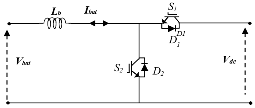
The bidirectional DC/DC converter enables power flow between two independent DC sources, facilitating energy exchange in either direction [22, 23]. Functioning as a dual-mode buck-boost converter, this topology allows for current reversal while maintaining consistent voltage levels at the terminals. The converter operates in two distinct modes:
1. Boost mode (discharge): In this configuration, energy is transferred from the battery to the DC bus [13]. During the first switching period, the IGBT S2 is activated, while in the second period, the freewheeling diode D1 conducts to maintain the current path.
2. Buck mode (charge): Conversely, when charging the battery from the DC bus, the converter operates in buck mode [13]. During the first period, IGBT S1 is gated on, and during the second period, diode D2 facilitates the freewheeling current.
The schematic representation of the bidirectional converter and its associated equivalent circuit are illustrated in Figure 5.
3.7 Battery energy storage modelling
In standalone PV pumping systems, the battery bank serves as a critical buffer, ensuring continuous power supply to the IM during daylight hours when the power generated by the PV array is insufficient to meet the load demand. Among the available electrochemical storage technologies, lead-acid batteries are predominantly utilized in such applications due to their proven reliability, cost-effectiveness, and established performance characteristics. The dynamic behaviour of the lead-acid battery is modelled using the semi-empirical approach, which relates the battery terminal voltage ($V_{bat}$) to the state of charge and discharge current [24]. The terminal voltage is defined by the following expressions for the charging and discharging modes, respectively.
Charging mode:
$V_{b a t}=v_0-R_i \cdot i+\exp (t)-K \frac{Q}{Q-i_t} i_t-K \frac{Q}{i_t-0.1 Q} i^*$ (38)
Battery discharging mode:
$V_{b a t}=v_0+\exp (t)-R_i \cdot i-K \frac{Q}{Q-i_t}\left(i_t+i^*\right)$ (39)
where, $V_{bat}$ is battery voltage $(V) ; v_0$ is constant voltage of battery $(V) ; Q$ is battery capacity $(A h) ; i_t$ is actual battery charge ($A h$); $R_i$ is internal resistance ($\Omega$); $K$ is polarization constant $(V /(A h)) ; i$ is current of the battery $(A)$ and $i^*$ is filtered current (A).
The proposed control architecture is organized into three hierarchical levels to ensure global system stability and optimal power distribution within the standalone PV pumping system.
4.1 Maximum power point tracking control
4.1.1 Variable step size perturb and observe
In conventional P&O algorithms, a fixed step size creates an inherent trade-off between tracking speed and steady-state accuracy. Large perturbations allow for rapid convergence during transient conditions but result in significant power oscillations around the MPP during steady-state operation. Conversely, small perturbations minimize these oscillations but lead to sluggish response times during atmospheric changes. Table 2 summarizes the operational logic, illustrating the relationship between perturbation direction, the resulting change in power, and the necessary corrective actions to converge toward the MPP [6, 7].
Table 2. The perturb and observe (P&O) maximum power point tracking (MPPT) algorithm operating principle
|
Position |
Variation |
Action |
|
1 |
$d P=0$ |
Noaction |
|
2 |
$+d P /+d V$ |
Increase $\Delta V$ |
|
3 |
$+d P /-d V$ |
Decrease $\Delta V$ |
|
4 |
$-d P /-d V$ |
Increase $\Delta V$ |
|
5 |
$-d P /+d V$ |
Decrease $\Delta V$ |
To overcome the limitations of the fixed-step approach, this study employs a variable step-size method. In the conventional P&O process, the reference voltage update is defined by a constant step size, $\Delta V$, as shown in Eq. (40):
$V_{\text {ref }}(k)=V_{\text {ref }}(k-1) \pm \Delta V$ (41)
To achieve an optimal balance between tracking rapidity and steady-state precision, a variable step-size approach is implemented. The proposed algorithm adjusts the step size dynamically based on the current operating point relative to the MPP. The update mechanism is defined in Eq. (41) [6]:
$V_{r e f}(k)=V_{r e f}(k-1) \pm N f(P, V)$ (42)
In this formulation, N represents a scaling factor—a constant parameter determined during the design phase—which dictates the overall performance characteristics and sensitivity of the MPPT system.
In this study, the variable step size used to solve the MPPT problem is shown as Eq. (42):
$V_{r e f}(k)=V_{r e f}(k-1) \pm N\left|\frac{\Delta P}{\Delta V}\right|$ (42)
4.1.2 Variable step size perturb and observe optimized by backstepping approach
To integrate the variable step-size P&O algorithm with backstepping control, we utilize the boost converter's dynamic model. The system is modelled by the state-space equations:
$C_1 V_{p v}=I_{p v}-I_L$ (43)
$L .I_L=V_{p v}-d^{\prime} V_0$ (44)
where, $d^{\prime}=(1-d)$ (with $d$ representing the duty cycle).
The backstepping design is performed in two sequential steps to ensure global asymptotic stability based on Lyapunov theory.
Step 1: Voltage Regulation (Outer Loop)
The voltage tracking error is defined as:
$e_1=V_{p v}-V_{r e f}$ (45)
Using the Lyapunov candidate $V_1=\frac{1}{2} e_1^2$, the stability condition is satisfied:
$\dot{V}_1=-k_1 e_1^2<0 \quad\left(\right.$ for $\left.k_1>0\right)$ (46)
By defining the virtual reference current $I_{ref}$:
$I_{r e f}=k_1 C_1 e_1+I_{p v}-C_1 \dot{V}_{r e f}$ (47)
Step 2: Current Regulation (INNER LOOP)
The current tracking error is defined as:
$e_2=I_L-I_{r e f}$ (48)
By constructing the augmented Lyapunov function $V_2=$ $V_1+\frac{1}{2} e_2^2$, we derive the final control law for the boost converter:
$d^{\prime}=\frac{L}{V_{d c}}\left[\frac{V_{p v}}{L}-\frac{e_1}{C_1}+k_2 e_2-k_1 C_1 e_1+I_{p v}+C_1 \dot{V}_{r e f}\right]$ (49)
This control law ensures that the derivative of the Lyapunov function guaranteeing that the system is globally asymptotically stable for positive gains $k_1$ and $k_2$:
$\dot{V}_2=-k_1 e_1^2-k_2 e_2^2<0$ (50)
The P&O algorithm serves as the outer loop, generating the reference voltage $V_{ref}$. The backstepping controller then acts as the inner regulation mechanism to force the system states toward this reference. This hybrid structure provides several advantages for high-performance PV systems:
Stability: The backstepping framework provides formal stability proofs, ensuring the converter tracks the P&O-generated reference without the instability common in standard linear controllers under varying conditions.
Dynamic response: By decoupling the voltage and current loops, the system achieves rapid response to climatic changes, which is effectively complemented by the variable step-size logic that minimizes steady-state oscillations around the MPP.
The design maintains stable performance despite parameter variations and load changes, as confirmed by simulation tests in Matlab/SimPowerSystems.
4.2 Nonlinear backstepping control of the induction motor
The association of the suggested backstepping controller is as described below:
$\left(\begin{array}{l}e_1=x_{11}^*-x_{11} \\ e_3=x_{21}^*-x_{21}\end{array}\right.$ (51)
Then, the error dynamical equations are:
$\left( \begin{array}{*{35}{l}} \overset{\bullet }{\mathop{e}}\,_{1}^{{}}=\overset{\bullet }{\mathop{x}}\,_{11}^{*}-2\frac{pL_{m}^{{}}}{JL_{r}^{{}}}x_{12}^{{}}+\frac{p}{J}Tl \\ \overset{\bullet }{\mathop{e}}\,_{3}^{{}}=\overset{\bullet }{\mathop{x}}\,_{21}^{*}+2\frac{R_{r}^{{}}}{L_{r}^{{}}}x_{21}^{{}}-2\frac{R_{r}^{{}}L_{m}^{{}}}{L_{r}^{{}}}x_{22}^{{}} \\\end{array} \right.$ (52)
$V=\frac{1}{2} e_1^2+\frac{1}{2} e_3^2$ (53)
$\begin{aligned} \dot{V} & =\dot{e}_1 e_1+\dot{e}_3 e_3 \\ = & e_1\left[\dot{x}_{11}^*-\frac{p L_m}{JL_r} x_{12}+\frac{p}{J} Tl \right]+e_3\left[\dot{x}_{21}^*+2 \frac{R_r}{L_r} x_{21}-2 \frac{R_r L_m}{L_r} x_{22}\right] \\ = & -k_1 e_1^2-k_3 e_3^2+e_1\left[k_1 e_1+\dot{x}_{11}^*-\frac{p L_m}{JL_r}+\frac{p}{J} T l\right] \\ & +e_3\left[k_3 e_3+2 \frac{R_r}{L_r} x_{21}-2 \frac{R_r L_m}{L_r} x_{22}\right]\end{aligned}$ (54)
$\left(\begin{array}{l}x_{12}^*=\frac{J L_r}{p L_m}\left[k_1 e_1+\dot{x}_{11}^*+\frac{p}{J} T l\right] \\ x_{22}^*=\frac{L_r}{2 R_r L_m}\left[k_3 e_3+2 \frac{R_r}{L_r} x_{21}\right]\end{array}\right.$ (55)
$\dot{V}=-k_1 e_1^2-k_3 e_3^2 \leq 0$ (56)
$\begin{aligned} e_2 & =x_{12}^*-x_{12} =\frac{J L_r}{p L_m}\left[k_1 e_1+\dot{x}_{11}^*\right]+\frac{J L_r}{p L_m} T l-x_{12}\end{aligned}$ (57)
$\begin{aligned} e_4 & =x_{22}^*-x_{22} =\frac{L_r}{2 R_r}\left[k_3 e_3+2 \frac{R_r}{L_r} x_{21}\right]-x_{22}\end{aligned}$ (58)
The error formulae in Eq. (51) can then be represented as follows:
$\left(\begin{array}{l}\dot{e}_1=-k_1 e_1+\frac{p L_m}{J L_r} e_2 \\ \dot{e}_3=-k_3 e_3+\frac{2 R_r}{L_r} e_4\end{array}\right.$ (59)
The dynamic equation for the error signals e2 and e4 can be calculated as follows:
$\left(\begin{array}{l}\dot{e}_2=\varphi_1-v_1 \\ \dot{e}_4=\varphi_2-v_2\end{array}\right.$ (60)
Such as, φ1 and φ2 are expressed as follows:
$\varphi _{1}^{{}}=\frac{JL_{r}^{{}}}{pL_{m}^{{}}}k_{1}^{{}}\left( -k_{1}^{{}}e_{1}^{{}}+\frac{pL_{m}^{{}}}{JL_{r}^{{}}}e_{2}^{{}} \right)+\frac{JL_{r}^{{}}}{pL_{m}^{{}}}\overset{\bullet \bullet }{\mathop{x}}\,_{11}^{*}+\frac{JL_{r}^{{}}}{pL_{m}^{{}}}\overset{\bullet }{\mathop{T}}\,l+\frac{R_{r}^{{}}}{L_{r}^{{}}}x_{12}^{{}}$ (61)
$\varphi_2=\frac{L_r}{p R_r} k_3\left(-k_3 e_3+2 \frac{R_r}{L_r} e_4\right)-2 \frac{R_r}{L_r} x_{21}+\frac{R_r}{L_r}\left(2 L_m+1\right) x_{22}$ (62)
The Lyapunov function presented in Eq. (53) is now extended to incorporate the state variables e2 and e4, expressed as:
$V_e=\frac{1}{2}\left(e_1^2+e_2^2+e_3^2+e_4^2\right)$ (63)
The Lyapunov function Ve serves as the basis for deriving the control algorithm. Accordingly, its derivative is recalculated in conjunction with the error dynamics defined by Eqs. (59)–(62):
$\begin{aligned} & \dot{V}_e=e_1 \dot{e}_1+e_2 \dot{e}_2+e_3 \dot{e}_3+e_4 \dot{e}_4 \\ = & e_1\left(-k_1 e_1+\frac{p L_m}{JL_r} e_2\right)+e_2\left(\varphi_1-v_1\right)+e_3\left(-k_3 e_3+2 \frac{R_r}{L_r} e_4\right)+e_4\left(\varphi_2-v_2\right) \\ = & -k_1 e_1^2-k_2 e_2^2-k_3 e_3^2-k_4 e_4^2+e_2\left[\frac{p L_m}{JL_r} e_1+k_2 e_2+\varphi_1-v_1\right] \\ & +e_4\left[2 \frac{R_r}{L} e_3+k_4 e_4+\varphi_2-v_2\right]\end{aligned}$ (64)
Based on the above analysis, the control laws are derived as follows:
$\left( \begin{array}{*{35}{l}} v_{1}^{{}}=\frac{pL_{m}^{{}}}{JL_{r}^{{}}}e_{1}^{{}}+k_{2}^{{}}e_{2}^{{}}+\varphi _{1}^{{}} \\ v_{2}^{{}}=2\frac{R_{r}^{{}}}{L_{r}^{{}}}e_{3}^{{}}+k_{4}^{{}}e_{4}^{{}}+\varphi _{2}^{{}} \\\end{array} \right.$ (65)
From the preceding expression, the control laws are formulated as follows, leading to:
$\dot{V}_e=-k_1 e_1^2-k_2 e_2^2-k_3 e_3^2-k_4 e_4^2 \leq 0$ (66)
$\left( \begin{array}{*{35}{l}} \phi _{s\alpha }^{{}}=\int{(u_{s\alpha }^{{}}}-R_{s}^{{}}i_{s\alpha }^{{}})dt \\ \phi _{s\beta }^{{}}=\int{(u_{s\beta }^{{}}}-R_{s}^{{}}i_{s\beta }^{{}})dt \\\end{array} \right.$ (67)
The rotor flux components φrα, φrβ can then be directly determined using:
$\left(\begin{array}{l}\phi_{r \alpha}=\frac{L_r}{L_m}\left(\phi_{s \alpha}-\sigma L_s i_{s \alpha}\right) \\ \phi_{r \beta}=\frac{L_r}{L_m}\left(\phi_{s \beta}-\sigma L_s i_{s \beta}\right)\end{array}\right.$ (68)
From Eq. (29), it is possible to compute $\omega_s^*$ as follows:
$\omega_s^*=\omega_m+\frac{\phi_{r q} v_2+\phi_{r d} v_1}{i_{s d} x_{21}}$ (69)
4.3 Control strategy for bidirectional DC-DC converter
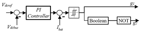
Figure 6 shows the proposed battery controller. To ensure stable operation of the bidirectional converter, a dual-loop control architecture is implemented. A Proportional-Integral (PI) controller is utilized to regulate the DC-link voltage by adjusting the power flow based on the DC bus reference. Concurrently, a hysteresis current controller is employed to manage the battery charging and discharging currents, providing rapid dynamic response and reliable stability against parameter variations. The tracking error for the DC bus voltage, $e_{V d c}$, and the battery current, $e_{Ibat}$, are defined by Eqs. (70) and (71), respectively:
$e_{V_{d c}}(k)=V_{d c, \text { ref }}-V_{d c}(k)$ (70)
$e_{V_{d c}}(k)=V_{d c, \text { ref }}-V_{d c}(k)$ (71)
Figure 6. The proposed bidirectional buck-boost controller under Simulink/MATLAB
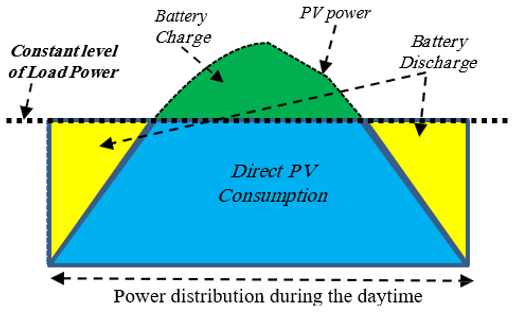
Figure 7. Battery operating modes
A primary objective of this design is to optimize the energy storage system. Given that battery banks are characterized by high capital expenditure, significant weight, and a service life approximately one-fifth that of PV modules, minimizing their capacity is critical for system sustainability. Consequently, the proposed system is optimized for daytime-only operation, as illustrated in Figure 7. During daylight hours, the PV array supplies the load and powers the water-pumping system. Instead of relying on electrochemical storage during nighttime hours, the system utilizes the potential energy of the stored water. This "water-as-battery" approach effectively shifts the storage requirement from electrical to mechanical potential energy, significantly extending the system’s overall operational lifespan and reducing maintenance costs.
To demonstrate the superior performance of the proposed VSS-P&O MPPT algorithm with a backstepping-based boost converter controller, coupled with a nonlinear backstepping controller utilizing the multi-scalar machine model for the IM drive fed by standalone PV-battery system, numerical simulations are implemented under Simulink/MATLAB. This control architecture is specifically engineered to provide high stability against parameter variations, load torque disturbances, and rapid atmospheric transitions. The scheme block diagram of the proposed controller is presented in Figure 1. The parameters of the verified motor are listed in Table 3. In this system, eight similar PV modules are associated in series and 6 batteries are connected in series; the specifications of PV panel and battery are shown in Tables 4 and 5, respectively.
Table 3. The induction motor (IM) parameters
|
Power |
1.5 [kw] |
|
Voltage |
400-230 [V] |
|
Stator resistance |
4.85 [Ω] |
|
Stator inductance |
0.274 [H] |
|
Rotor resistance |
3.805 [Ω] |
|
Rotor inductance |
0.274 [H] |
|
Mutual inductance |
0.258 [H] |
|
Rotor inertia |
0.031 [kg.m2] |
|
Friction coefficient |
0.008 [N.s/rd] |
|
Number of pole pairs |
2 |
Table 4. Panel parameters
|
Open circuit voltage |
37.9 [V] |
|
Short circuit current |
9.07 [A] |
|
Optimal voltage |
30.8 [V] |
|
Optimal current |
8.77[ A] |
|
Maximum power |
270 [W] |
Table 5. Batteries parameters
|
Type |
Lead-acid |
|
Number of batteries |
6 |
|
Nominal voltage |
24 V |
|
Initial SoC |
60 % |
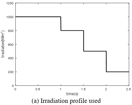
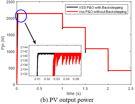
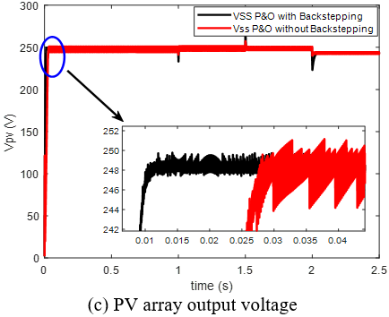
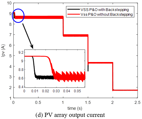
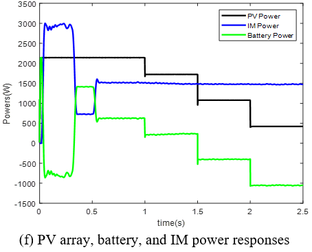
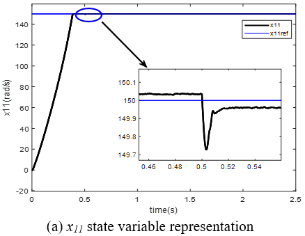
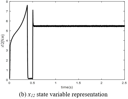
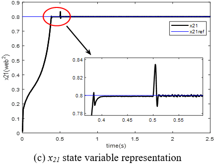
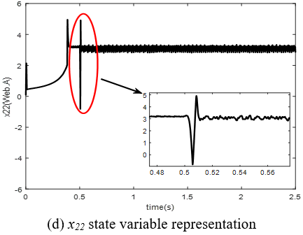
Figures 8 and 9 evaluate the system’s dynamic performance of the IM drive subjected to simultaneous fluctuations in solar irradiance and mechanical loading. As illustrated in the irradiance profile in Figure 8(a), the system was subjected to a staircase-downward sequence of step changes—transitioning from 1000 W/m² to 800 W/m², then to 500 W/m², and finally to 200 W/m² — to simulate rapid atmospheric instability. To further challenge the controller's disturbance rejection capabilities, the motor speed reference x11 was maintained at a constant 150 rad/s, while a step load torque of 5 N.m was abruptly applied at t = 0.5 s. This rigorous simulation scenario validates the ability of the proposed nonlinear backstepping controller to decouple mechanical load disturbances from the primary power-tracking objectives. Figures 8 and 9 demonstrate the dynamic response of the system and the performance of the IM under rapid variations in solar irradiation and load conditions. Figure 8(a) depicts the irradiation profile, which transitions from 1000 W/m² to 800 W/m², then to 500 W/m², and finally to 200 W/m². Concurrently, the speed reference (x11) is set to 150 rad/s during the entire simulation time, at t = 0.5 s, a load torque of 5 N.m is applied.
Figure 8. Energy performance of the system
Figure 9. Dynamic response of the multi-scalar control variables (x11, x12, x21, x22) during irradiance and load torque transitions
5.1 Comparative analysis: Variable-step-size-perturb and observe vs. variable-step-size-perturb and observe with backstepping
When comparing the performance of the standard VSS-P&O against the proposed VSS-P&O integrated with the backstepping controller, the results underscore a significant improvement in tracking efficiency (as listed in Table 6).
Table 6. Maximum power point tracking (MPPT) comparison techniques
|
Insolation Level |
Strategy |
1000 W/m² |
800 W/m² |
500 W/m² |
200 W/m² |
|
Power (W) |
A |
2139.3 |
1720.17 |
1076.08 |
420.97 |
|
B |
2141.16 |
1721.58 |
1076.63 |
421.04 |
|
|
Settling time (s) |
A |
0.03 |
0.003 |
0.06 |
0.002 |
|
B |
0.01 |
0.002 |
0.04 |
0.02 |
|
|
Power ripple (W) |
A |
4.88 |
2.82 |
1.09 |
0.07 |
|
B |
0.1 |
0.08 |
0.025 |
0.01 |
|
|
Efficiency (%) |
A |
99.04 |
99.54 |
99.63 |
97.44 |
|
B |
99.13 |
99.63 |
99.68 |
97.46 |
Dynamic convergence: While the standard VSS-P&O exhibits successful tracking of the MPP, the inclusion of the backstepping controller significantly reduces the settling time during rapid irradiance transients.
Stability: The backstepping controller suppresses the high-frequency "chattering" or oscillations often present in standalone P&O methods, ensuring a smoother transition between operating points on the P−V curve.
5.2 DC bus voltage stability
The DC bus voltage response under the proposed control strategy demonstrates the ability to maintain stability despite external disturbances.
Performance: With a reference Vdc,ref = 515 V, the voltage maintains high stability throughout varying irradiance profiles (1000 to 200 W/m2).
Control Synergy: The minimal voltage ripple observed confirms that the backstepping controller effectively decouples the boost converter's internal states from load-side fluctuations, providing a stable voltage source for the IM drive.
5.3 Power flow and operational modes
The power distribution among the PV array, battery bank, and IM drive illustrates the system’s adaptive energy management.
PV Array Power: Tracks the available solar energy with near-instantaneous response times, proving the effectiveness of the VSS-P&O optimization.
Battery Power Management: The system seamlessly switches between buck mode (charging) when Ppv > Pload and boost mode (discharging) when Ppv < Pload.
IM Drive Power: Remains consistent with demand, as the bidirectional power flow ensures that the motor receives a steady power supply regardless of solar variability.
5.4 Multi-Scalar Variables of the induction motor
Table 7. Motor speed comparison techniques
|
Control Technique |
Average Speed (rad/s) |
Settling Time (s) |
Speed Ripple (rad/s) |
|
Backstepping |
157.03 |
0.38 |
0.005 |
|
Classical PI |
156.95 |
0.7 |
0.15 |
Table 8. Control parameters
|
Controller |
Parameter |
|
VSS-P&O MPPT |
Vpv(kp, ki) = (7.46, 0.1772); IL (kp, ki) = (10, 0.001) |
|
Backstepping MPPT |
k1 = k2 = 500 |
|
DC bus voltage |
Vdc (kp, ki) = (2.12, 450) |
|
Non-linear control of IM using backstepping |
k1 = k3 = 900; k2 = k4 = 1200. |
|
Non-linear control of IM using classical PI |
x11(kp, ki) = (0.1933, 1.1852); x12(kp, ki) = (545.7, 320000); x21(kp, ki) = (6.57, 313.3816); x22(kp, ki) = (545.7, 320000); |
The multi-scalar control approach utilizes the state variables (x11, x12, x21, x22) to decouple the motor dynamics.
Trajectory Tracking: The variables x21 and x22 (representing flux-related states) maintain precise tracking of their references (x21 = 0.8 Wb2), demonstrating that the multi-scalar model effectively handles nonlinearities.
The variables x11 and x12 (torque-related states) exhibit resilience to load torque variations. The smooth evolution of these variables confirms that the IM drive operates efficiently and rejects disturbance, validating the use of the nonlinear backstepping technique over classical linear PI-based approaches (as compared in Table 7, with the respective controller tuning parameters detailed in Table 8).
5.5 Characteristics of standalone photovoltaic water pumping system for one day
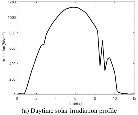
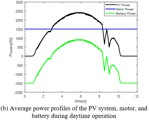
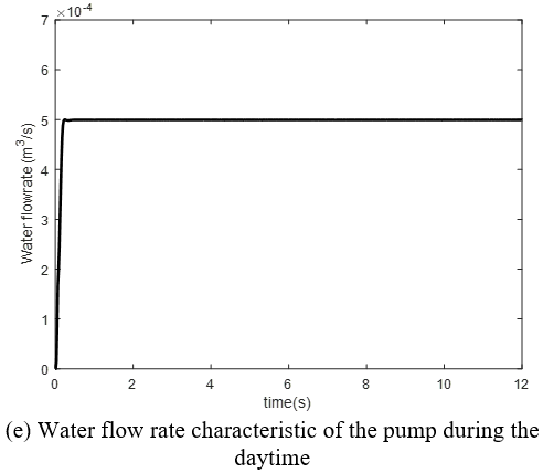
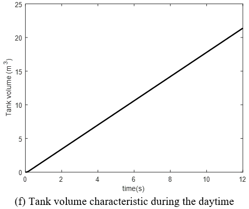
The dynamic daily performance of the SPVWPS is illustrated in Figure 10 through its core electrical, thermal, and mechanical operating profiles over a 12-hour period of daytime from 7 AM to 7 PM. This evaluation is based on a maximum tank volume of 50 m3 and an average daily water demand of 18 m3/day.
Solar Irradiation Profile (Figure 10(a)): Demonstrates the diurnal solar availability, following a standard bell curve that rises from zero at sunrise, reaches its peak irradiance S = 1180 W/m2 at solar noon, and declines back to zero at sunset.
Average Power Profiles (Figure 10(b)): Highlights the energy distribution and power flow between system components:
PV System Output: Directly tracks the solar irradiation profile, reaching maximum power delivery during daylight hours.
Motor Power: Maintains a stable around 1.5 kW, regulated input required to operate the pump efficiently at nominal speed of 157 rad/s and nominal motor torque about 11 N.m, absorbing available PV power and utilizing the energy storage system during generation dips.
Battery Power: Acts as a buffer, charging during periods when PV power exceeds motor demand and discharging to supplement the motor when solar irradiation drops below operational thresholds or during transient cloud coverage.
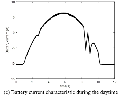
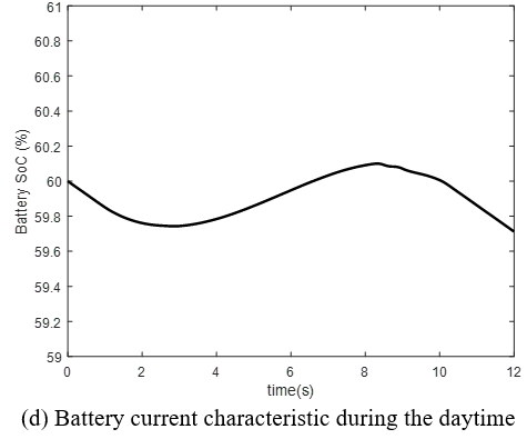
Battery Current and SoC Characteristics (Figure 10(c) and (d)): Reflect the bidirectional current flow of the storage unit:
State of Charge (SoC): The battery SoC begins at an initial value of 60%, initially decreasing while PV power is less than load demand. It reaches 59.743% when PV power matches the motor-pump demand, after which the battery bank begins charging until SoC reaches 60.1% as PV power again meets load requirements. It then enters a final discharging phase as solar generation decreases, ending at an SoC of 59.71% at 7:00 PM.
Positive Current (Charging): Peaks at 6.375 A during midday when solar generation exceeds the pump's immediate power demand. This excess PV energy is directed into the battery bank to recharge it and preserve energy for low-irradiance conditions.
Negative Current (Discharging): Occurs during early morning, late afternoon, or sudden irradiance drops to sustain continuous pump operation.
Water Flow Rate Characteristic (Figure 10(e)): The water flow rate was fixed at Q = 5 × 10⁻⁴ m³/s based on a constant motor speed of 157 rad/s, allowing the system to operate at its maximum available power.
Tank Volume Characteristic (Figure 10(f)): This graph illustrates the cumulative water storage over time. The tank volume increases continuously throughout the 12 hours of daylight as the pump operates, reaching maximum capacity of V = 21.39 m3 by late afternoon (7:00 PM) to provide a reliable water buffer during periods of zero irradiance.
Figure 10. Operating profile of the standalone photovoltaic water pumping system (SPVWPS) during the daytime
The proposed system utilizes a dual-layer control strategy to effectively address the inherent challenges typically encountered in standalone PV-powered IM drives. By integrating a VSS-P&O MPPT algorithm—which is designed through a backstepping control framework—the system achieves rapid, high-precision power extraction that is highly resilient to environmental volatility. Furthermore, by adopting an innovative “water-as-battery” approach, the design fundamentally mitigates the drawbacks traditionally associated with conventional electrochemical storage systems, which are known to be prone to degradation and have a lifespan significantly shorter than that of PV modules. The key aspects of this longevity-focused design include: 1) Electrochemical battery usage is strategically optimized by relying on potential energy storage (water pumping) during the night, thereby effectively reducing the battery bank’s cyclic load and extending its operational life. 2) The incorporation of a multi-scalar IM model within the nonlinear backstepping control architecture ensures stable and efficient motor performance, even under extreme fluctuations in irradiance. 3) As clearly demonstrated by the simulation results, the seamless transition between buck and boost modes ensures that both the DC bus voltage and motor speed tracking remain stable regardless of the actual power flow direction.
This integrated approach not only optimizes the energy conversion process but also significantly lowers long-term maintenance costs and improves the overall sustainability of the pumping system for standalone applications.
|
IM |
Induction motor |
|
MPPT |
Maximum power point tracking |
|
MPP |
Maximum power point |
|
P&O |
Perturb and observe |
|
VSS |
Variable step size |
|
PV |
Photovoltaic |
|
SPVWPS |
Standalone photovoltaic water pumping system |
|
SoC |
State of charge |
|
FOC |
Field-oriented vector control |
|
Q |
Water flow rate |
|
V |
Tank volume |
[1] Almihat, M.G.M., Munda, J.L. (2025). The role of smart grid technologies in urban and sustainable energy planning. Energies, 18(7): 1618. https://doi.org/10.3390/en18071618
[2] Sontake, V.C., Kalamkar, V.R. (2016). Solar photovoltaic water pumping system-A comprehensive review. Renewable and Sustainable Energy Reviews, 59: 1038-1067. https://doi.org/10.1016/j.rser.2016.01.021
[3] Villalva, M.G., Gazoli, J.R., Ruppert Filho, E. (2009). Comprehensive approach to modeling and simulation of photovoltaic arrays. IEEE Transactions on Power Electronics, 24(5): 1198-1208. https://doi.org/10.1109/TPEL.2009.2013862
[4] Hanzaei, S.H., Gorji, S.A., Ektesabi, M. (2020). A scheme-based review of MPPT techniques with respect to input variables including solar irradiance and PV arrays’ temperature. IEEE Access, 8: 182229-182239. https://doi.org/10.1109/ACCESS.2020.3028580
[5] Logeswaran, T., SenthilKumar, A. (2014). A review of maximum power point tracking algorithms for photovoltaic systems under uniform and non-uniform irradiances. Energy Procedia, 54: 228-235. https://doi.org/10.1016/j.egypro.2014.07.266.
[6] Abdelsalam, A.K., Massoud, A.M., Ahmed, S., Enjeti, P.N. (2011). High-performance adaptive perturb and observe MPPT technique for photovoltaic-based microgrids. IEEE Transactions on Power Electronics, 26(4): 1010-1021. https://doi.org/10.1109/TPEL.2010.2089645
[7] Kchaou, A., Naamane, A., Koubaa, Y., M’sirdi, N. (2017). Second order sliding mode-based MPPT control for photovoltaic applications. Solar Energy, 155: 758-769. https://doi.org/10.1016/j.solener.2017.07.007
[8] Kokotovic, P.V. (1992). The joy of feedback: Nonlinear and adaptive. IEEE Control Systems Magazine, 12(3): 7-17. https://doi.org/10.1109/37.165507
[9] Ali, K., Khan, Q., Ullah, S., Khan, I., Khan, L. (2020). Nonlinear robust integral backstepping based MPPT control for stand-alone photovoltaic system. PLOS One, 15(5): e0231749. https://doi.org/10.1371/journal.pone.0231749
[10] Ali, K., Khan, L., Khan, Q., et al. (2019). Robust integral backstepping based nonlinear MPPT control for a PV system. Energies, 12(16): 3180. https://doi.org/10.3390/en12163180
[11] Ballouti, A., Chouiekh, M., Ameziane, H., et al. (2026). Bioinspired STHVO based MPPT control for grid connected photovoltaic water pumping systems. Scientific Reports, 16(1): 4866. https://doi.org/10.1038/s41598-026-35176-3
[12] Singh, K.K., Thakur, R. (2026). Grid-integrated rooftop solar water pumping using BLDC motor drive. In 2026 International Conference on Electrical and Electronics for Sustainable Innovations (ICEESI), Raigarh, India, pp. 1-6. https://doi.org/10.1109/ICEESI68020.2026.11583050
[13] Benbaha, N., Zidani, F., Said, M.S.N., Eddine Boukebbous, S., Ammar, H. (2017). Optimal energy control of induction motor standalone photovoltaic battery pumping system. In 2017 6th International Conference on Systems and Control (ICSC), Batna, Algeria, pp. 622-628. https://doi.org/10.1109/ICoSC.2017.7958685
[14] Gevorkov, L., Domínguez-García, J.L., Romero, L.T. (2022). Review on solar photovoltaic-powered pumping systems. Energies, 16(1): 94. https://doi.org/doi: 10.3390/en16010094
[15] Vas, P. (1990). Vector Control of AC Machines. Oxford University Press.
[16] Bose, B.K. (2002). Modern Power Electronics and AC Drives: Limitations of Scalar Frameworks and Evolution of Vector Topologies. Prentice Hall.
[17] Blaschke, F. (1772). The principle of field orientation as applied to the new transvector closed-loop control system for rotating-field machine. Siemens Review, 34: 217-220.
[18] Marino, R., Peresada, S., Valigi, P. (1993). Adaptive input-output linearizing control of induction motors. IEEE Transactions on Automatic Control, 38(2): 208-221. https://doi.org/10.1109/9.250510
[19] Uyulan, C. (2019). A robust-adaptive linearizing control method for sensorless high precision control of induction motor. Measurement and Control, 52(5-6): 634-656. https://doi.org/10.1177/0020294019833072
[20] Krzemiński, Z. (1987). Nonlinear control of induction motor. IFAC Proceedings Volumes, 20(5): 357-362. https://doi.org/10.1016/S1474-6670(17)55396-3
[21] Mehazzem, F., Nemmour, A.L., Reama, A. (2017). Real time implementation of backstepping-multiscalar control to induction motor fed by voltage source inverter. International Journal of Hydrogen Energy, 42(28): 17965-17975. https://doi.org/10.1016/j.ijhydene.2017.05.035
[22] Wogi, L., Morawiec, M., Ayana, T., Kołodziejek, P. (2025). Multiscalar control-based flux optimization for efficiency improvement of induction motor. IEEE Transactions on Transportation Electrification, 11(6): 14047-14061. https://doi.org/10.1109/TTE.2025.3606829
[23] Dastgiri, A., Hosseinpour, M., Yazdi, S., Seifi, A. (2026). Design and control of a high-voltage-gain four-port DC-DC converter with efficient bidirectional energy storage for renewable energy applications. IEEE Access, 14: 123880-123909. https://doi.org/10.1109/ACCESS.2026.3722218
[24] Benbaha, N., Zidani, F., Nait-Said, M.S., Zouzou, S.E., Boukebbous, S., Ammar, H. (2018). DSPACE validation of improved backstepping optimal energy control for photovoltaic systems. In 2018 6th International Renewable and Sustainable Energy Conference (IRSEC), Rabat, Morocco, pp. 1-6. https://doi.org/10.1109/IRSEC.2018.8702908