Mohammed Younis Thanoun* | Mohammad J. M. Zedan | Abdulbasit M. A. Sabaawi | Ahmed A. Mohammed | Ersin Elbasi | Mohd Asyraf Zulkifley
© 2026 The authors. This article is published by IIETA and is licensed under the CC BY 4.0 license (http://creativecommons.org/licenses/by/4.0/).
OPEN ACCESS
Reliable transmission of medical images over wireless networks is essential for modern telemedicine, yet the impact of channel impairments on deep-learning segmentation accuracy remains underexplored. In this work, HUM-Net, a hybrid U-shaped architecture, is proposed by integrating convolutional encoders with a Mamba-based Visual State Space (VSS) bottleneck and State-Space Attention Gates (SSAG) for kidney tumor segmentation in CT imagery. To evaluate its robustness under controlled physical-layer conditions, an end-to-end physical-layer simulation framework is developed by subjecting each image to representative wireless degradations, including Joint Photographic Experts Group (JPEG) source coding (Q = 10–70), Gilbert–Elliott packet loss (0.1%–10%), additive white Gaussian noise (Eb/N0 = 0–30 dB), and four representative combined-stress conditions. Using the KiTS23 dataset (6,289 curated 512 × 512 slices), HUM-Net is evaluated on more than 30,000 degraded images covering 24 distinct channel conditions. HUM-Net achieves a baseline Dice Score (DSC) of 0.9562 and mean Intersection-over-Union (mIoU) of 0.9569, while remaining highly robust to lossy compression. Furthermore, noise above 10 dB Eb/N0 is fully recoverable, while severe noise (0 dB) reduces the DSC to 0.7116. Packet loss, however, is severely disruptive: DSC drops to 0.8848 at just 0.2% loss and to 0.5275 at 1%. In combined-stress conditions, packet loss consistently dominates: DSC values track the packet-loss-only curve rather than the noise-only curve, and the two impairments interact only mildly (±2.6% DSC). Overall, these findings establish a clear hierarchy of impairments and indicate that, within the simulated conditions, packet-loss recovery warrants priority over compression mitigation and noise reduction in the design of wireless medical imaging links, subject to confirmation on deployed systems.
kidney tumor segmentation, Mamba, state-space models, wireless medical imaging, Joint Photographic Experts Group, packet loss, additive white Gaussian noise, deep learning robustness
Medical image segmentation has emerged as an essential component of computer-aided diagnosis, particularly for the early detection and quantitative analysis of solid tumors. Computed tomography (CT) is one of the radiological modalities whose resolution and contrast allow kidney lesions to be outlined, yet manual annotation of such images is tedious, observer-dependent, and increasingly impractical given the growing volume of imaging data worldwide. Recent deep-learning algorithms for segmentation have become a scalable alternative, reaching expert-level performance on benchmarks such as KiTS [1], LiTS [2], and BraTS [3]. These models are now increasingly deployed in distributed and mobile settings, such as 5G-enabled telemedicine, cloud-based radiology, and remote diagnostic services [4, 5]. They operate on imagery that has travelled through wireless networks before reaching the inference engine. Whether this transmission step affects the accuracy of state-of-the-art segmentation models remains an open and largely unaddressed question.
Long-range contextual modelling has recently been used to better delineate complex structures in medical segmentation models [6-9]. The VMamba [10] and U-Mamba [11] are examples of Mamba-based methods that provide alternative efficient options for this. However, these models are generally evaluated using pristine, locally stored images, leaving their reliability after realistic wireless transmission largely unknown. To overcome this limitation, HUM-Net uses a Visual State Space (VSS) bottleneck for modelling global dependencies and State-Space Attention Gates (SSAG) modules for selectively refining skip-connected features.
A high percentage of published evaluations are conducted on pristine images stored locally, implicitly assuming that the transmission channel is lossless and noise-free [12, 13]. In practice, wireless medical imaging traffic is subject to a range of impairments: lossy source coding to reduce bandwidth (e.g., Joint Photographic Experts Group (JPEG) and DICOM-JPEG2000 gateways), bit errors from additive thermal noise and fading, and packet erasures from congestion and handover events. Surveys of 5G healthcare deployments report end-to-end packet loss in the 0.1%–7.2% range under normal operation [4], with bit error rates (BER) that depend strongly on channel state, modulation, and coding. Most prior work has focused on isolated effects, such as the impact of JPEG quality on classification accuracy [14, 15] or additive Gaussian noise on natural-image classifiers [16, 17], but limited studies have simulated source coding, channel noise, and erasure loss within a single physically grounded configuration, and almost none have addressed medical segmentation.
This omission is consequential. Segmentation networks operate on dense, pixel-level predictions and are therefore far more sensitive to localised image corruption than classification or detection networks. A single dropped packet can erase a 4 × 4 image block and displace tumor boundaries by several pixels, and a low-bit-rate JPEG approximation can smooth precisely the edges that distinguish a lesion from healthy parenchyma. Moreover, different impairment types degrade images in qualitatively distinct ways: compression introduces structured frequency-domain artifacts, channel noise produces broadband random errors in the spatial domain, and packet loss creates spatially contiguous blank regions. Robustness of a given segmentation model to one impairment does not imply robustness to another, and the interaction between impairments under combined-stress conditions remains uncharacterized. Therefore, the reliability of model deployment for practical use in remote medical imaging systems requires consideration of transmission, as high accuracy on standard benchmark images may yield unreliable tumor boundaries after wireless transmission.
Motivated by these gaps, this paper introduces two interrelated contributions. First, we propose HUM-Net, a hybrid U-shaped segmentation network that combines a convolutional encoder–decoder with a Mamba-based VSS bottleneck and SSA, delivering superior kidney tumor segmentation compared with five established baselines on the KiTS23 dataset. The VSS bottleneck allows for efficient modelling of global spatial dependencies, and SSAG modules selectively refine spatial features of the skip-connected encoder to suppress irrelevant information and preserve the tumor-related spatial details. Second, we design and validate an end-to-end physical-layer simulation framework in which each segmented image is corrupted by realistic wireless channel degradations, namely: JPEG source coding, additive white Gaussian noise (AWGN), Gilbert–Elliott packet loss, and four combined-stress conditions within a single QPSK-based transmitter–receiver pipeline that incorporates root-raised-cosine (RRC) pulse shaping, pilot-aided LS channel estimation, and minimum mean-square-error (MMSE) equalisation. Within this framework, we evaluate HUM-Net across 24 distinct channel conditions covering more than 30,000 degraded images, and report the resulting segmentation accuracy in terms of Dice Score (DSC), mean Intersection-over-Union (mIoU), sensitivity, and HD95. The obtained results show that HUM-Net is highly resilient to aggressive lossy compression and to noise above 10 dB Eb/N0, yet is severely degraded by even modest packet loss. In combined-stress conditions, packet loss consistently dominates, with direct implications for the design of channel coding, retransmission, and packet-recovery strategies in wireless medical imaging systems.
The remainder of this paper is organised as follows. Section 2 reviews related work on medical image segmentation and on the robustness of deep models to perturbations in the image and transmission domains. Section 3 presents the proposed HUM-Net architecture, the physical-layer simulation framework, the dataset, and the experimental protocol. Section 4 reports the segmentation and channel-degradation results and discusses their implications for system design. Section 5 concludes the paper and outlines future work.
Modern healthcare systems rely on transmitting medical images over various communication networks for remote medical diagnosis. However, communication channels often introduce interference, including packet loss, compression distortions, and random noise, which reduces the quality of transmitted images and consequently affects subsequent tasks such as segmentation. Despite this, most studies still focus on developing medical image segmentation algorithms through various strategies, such as transformers, transfer learning, and attentional mechanisms, without considering the network-based medical imaging environment [18-21]. Thus, the literature is reviewed thematically, including state space segmentation, packet loss, compression, noise, and semantic communication.
Recent state-space solutions have enabled very efficient long-range dependency modelling in medical image segmentation. U-Mamba introduces convolutional feature extraction and selective state-space modelling to a self-configuring biomedical segmentation framework [11], while VM-UNet uses VSS blocks as key elements of a U-shaped encoder–decoder architecture [22]. Swin-UMamba also introduces an ImageNet pre-trained Mamba encoder and a medical-image segmentation decoder, showing that transfer learning is beneficial for state-space models (SSMs) [23]. Although these methods show good results, they are mainly tested on clean benchmark images without communication-induced image degradation. Hence, their improvements do not guarantee state-space segmentation is reliable during image transmission.
Regarding packet loss, several studies have examined its impact on medical diagnostic efficiency. Chuprov et al. [24] revealed that packet loss of 2–5% in transmitted X-ray images negatively affected deep-learning performance by approximately 20%. Similarly, Shiranthika et al. [25] observed a sharp decline in U-Net segmentation when data-loss rates became high. All of these studies show that packet loss can negatively affect medical-image analysis [26]. But due to the differences in imaging modality, task, range of lost packets, and loss-injection technique, direct comparison is not possible, and realistic packet erasures still have not been extensively explored for state-space segmentation.
Compression robustness has also been widely investigated. Chen et al. [27] employed JPEG and JPEG2000 techniques to study their impact on medical-image segmentation and detection, showing that substantial compression could preserve most task performance. El Khoury et al. [28] found that 3D U-Net was more resistant to pelvic CT compression than its 2D counterpart. The results suggest that moderate compression could help to retain task-relevant information while more aggressive compression could lead to the loss of important image information. In general, however, compression is not measured in a full communication chain, but in an isolated fashion.
Related studies have also explored the impact of added noise across communication channels [29-31]. Jiu et al. [30] reported performance deterioration in DeepLab, FPN, and U-Net after Gaussian noise was added to X-ray images, while Babaeipour et al. [32] found that enhanced vision-transformer models were more robust than conventional CNNs. In general, these studies show that robustness to noise is architecture-dependent and is related to the level of degradation of the content. Most, however, add the noise directly on top of the images without propagating the noise through modulation, channel estimation, equalisation, and reconstruction [33].
Semantic communication has also been considered as an efficient task-based method for image transmission through bandwidth-limited and noisy channels. Yuan et al. [34] designed a generative system combining image reconstruction and segmentation, while DiSC-Med used semantic representation and diffusion-based reconstruction for robust medical CT transmission [35]. These works, however, focus primarily on transmission efficiency, reconstruction quality, or communication-oriented segmentation, but fail to assess the strength of a medical segmentation network in the face of compression, AWGN, packet loss, and their combination. As a result, semantic communication research does not directly prove the robustness of an independently developed segmentation model against multiple physical layer impairments. The literature therefore focuses on a number of more or less distinct themes, such as the notion of state-space segmentation under clean conditions, robustness to the various types of degradation, and semantic communication for efficient transmission or reconstruction. There is a lack of systematic research to assess the reliability of a task-level medical segmentation model in a state-space framework for various physical-layer impairments.
3.1 Baseline segmentation models
In this work, 3D medical images are converted into 2D to facilitate processing and model training. Accordingly, a set of core image segmentation models was employed to understand the context of these images in various ways, aiming to accurately identify kidney tumor boundaries. Specifically, experiments were conducted using five deep learning segmentation models: U-Net, SEG-Net [36], FCNet [37], PSP-Net [38], and DeepLabV2 [39]. During the evaluation, several evaluation metrics were used to determine the best-performing model as listed in Table 1. On this basis, some parameters can be drawn to design the proposed structure, which will be designed to accurately capture tumor details at the pixel level.
Table 1. Architectural summary of the five baseline segmentation models
|
Model |
Architecture Type |
Encoder/Backbone |
Param (M) |
Model Size (MB) |
GFLOPs |
Inference Time (ms/Image) |
Peak GPU Memory (MB) |
|
U-Net |
Encoder–Decoder + skip connection |
Custom CNN |
31.04 |
124.17 |
90.03 |
59.58 |
1680 |
|
SEG-Net |
Encoder–Decoder + pooling indices |
VGG-like CNN |
29.47 |
112.5 |
80.10 |
61.33 |
1541 |
|
PSP-Net |
Pyramid pooling + CNN |
ResNet-50 |
46.58 |
186.4 |
147.6 |
82.25 |
2283 |
|
FCNet |
Fully Convolutional Network (FCN-8) |
VGG16 backbone |
131.3 |
525.1 |
221.7 |
97.13 |
2944 |
|
DeepLab V2 |
Atrous convolution + dilated CNN |
ResNet-101 |
44.6 |
178.1 |
177.2 |
102.9 |
2443 |
3.2 The proposed segmentation model
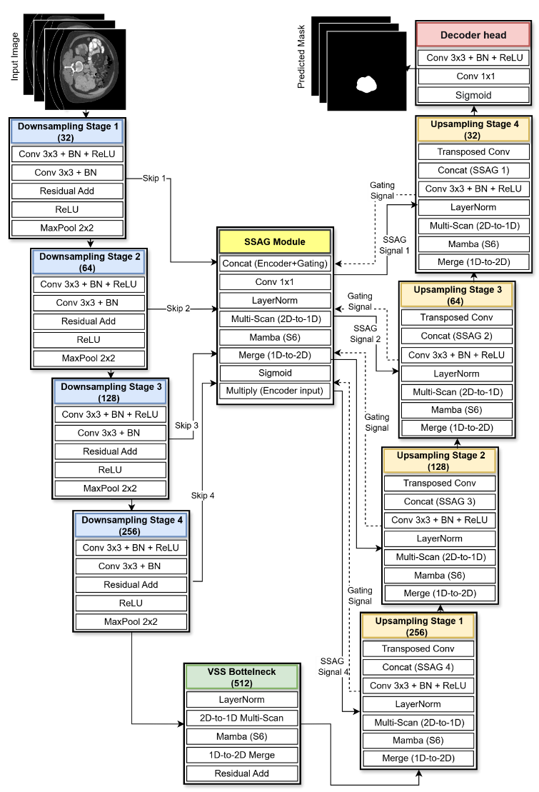
Based on findings gained from the benchmarking process, a novel approach was adopted, aiming to synergistically integrate convolutional neural networks used for extracting complex features with the Mamba framework. This framework is based on long-range dependency modeling of selective SSMs with limited computational complexity. The proposed approach, termed 'HUM-Net', follows a symmetrical encoder-decoder pattern ending in a dedicated bottleneck and linked by gated connections, as illustrated in Figure 1. HUM-Net is trained with a compact custom architecture with only about 8.95 million parameters and a storage demand of 34 MB. It was also analysed by the efficiency measures of FLOPs of 66.8, inference latency of 56.2 and peak GPU memory of 1280. This level of optimisation allows the design to be efficiently deployed on resource-constrained devices while also achieving outstanding results in segmentation.
Figure 1. The proposed segmentation model (HUM-Net)
3.2.1 HUM-Net encoder
The proposed encoder side is basically used to extract fine-grained hierarchical representations, including the complex texture and boundaries of the kidney tumors. The input CT image is defined as a tensor $\mathrm{X}=\in \mathrm{R}^{\mathrm{H} \times \mathrm{W} \times \mathrm{C}}$, where H and W represent the dimensions of the tensor while C represents the number of modalities. These images are passed to four successive levels of downsampling stages. Each stage includes a residual convolution block that reduces the spatial dimension of the tensor while doubling the channel capacity. The proposed convolutional blocks comprise two sets of 3 × 3 convolutions followed by batch normalisation and ReLU activations. The output of these sets is added to the residual connection from the input to prevent the vanishing gradient during the training phase. This process is concluded by pooling with a stride of 2 to reduce the dimension of the extracted features. By the fourth stage, the encoder produced highly abstracted feature maps with 16 × 16 × 8 dimensions.
3.2.2 The Visual State Space bottleneck
The proposed HUM-Net includes a bottleneck module that is built on the Mamba architecture. This module uses the VSS instead of the conventional convolution or attention blocks to effectively capture the global semantic relationship across the kidney body and the overlayed tumor. The VSS architecture was originally designed to work on 1D sequences, however the received tensors are 2D. To perform the matching, a 2D to 1D multi-scan mechanism is proposed to flatten the consecutive tensors by scanning across four directional routes. The resulting scans are passed to the Mamba selective scan algorithm (S6), which processes the received scans independently by compressing related context while neglecting the irrelevant background noise. After that, the processed scans are merged and reshaped to its original 2D spatial size and added with a residual connection to produce the bottleneck output that is passed to the decoder.
3.2.3 State-Space Attention Gate
This active module is proposed to link the encoder stages with the decoder using effective attention gates. These gates are used to selectively filter the high-resolution output from each stage of the encoder using gating signals generated by the reconstructed semantic features from the decoder. The encoder features and the gating signals are concatenated and passed to a 1 × 1 convolution. The output is then normalized, flattened and fed to the Mamba module, which continuously scan the spatial dimensions of tensors to find significant regions relevant to tumor class. Finally, the resulted output is reshaped to its original 2D spatial size and passed through a Sigmoid activation to generate continuous attention maps that multiplied with encoder input and passed to the decoder stages. This method guarantees that the decoder is rigorously supplied with boundary and texture data associated with the target class.
3.2.4 HUM-Net decoder
The decoder side progressively performs upsampling for the compressed features that resulted from the bottleneck module to eventually generate the pixelwise predictions with the original resolution. More specifically, in each stage of the decoder, the feature maps are upsampled by 2 using bilinear interpolation. After that, a concatenated process is applied with the gating signal and the results are passed to one set of standard 3 × 3 convolutions followed by normalisation and ReLU activation. Subsequently, a LayerNorm and Mamba operation are applied to re-evaluate the long-range spatial dependencies of the newly reconstructed features and prevent the loss of the global context even as the resolution increases during the upsampling process. Finally, the output of the fourth upsampling stage is delivered to the decoder head, which performs one set of 3 × 3 convolutions to refine the upsampled artefacts, accompanied by pointwise convolution and Sigmoid activation to densely predict the masks.
3.3 Wireless channel simulation framework
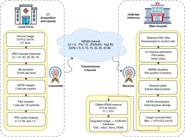
The robustness of the proposed HUM-Net is examined under controlled, physically grounded wireless transmission conditions through the development of an end-to-end physical-layer simulation framework. This framework applies a full transmitter–channel–receiver chain to every kidney CT image in the test set before the reconstructed image is passed to the segmentation network for inference. The framework operates at the bit level so that the effect of each physical-layer block on the recovered image can be measured directly. A complete overview of the pipeline is shown in Figure 2.
Figure 2. End-to-end physical-layer simulation framework used to evaluate HUM-Net robustness under wireless channel impairments
The simulation includes four independent degradation blocks and one combined-stress block. Block 1 evaluates the effect of lossy source coding over a clean transmission path using JPEG compression at five quality factors (Q = 70, 50, 30, 20, 10). Block 2 evaluates Gilbert–Elliott packet erasure at seven loss rates (0.1%, 0.2%, 0.5%, 0.75%, 1%, 5%, and 10%) with a fixed packet block size of 4 × 4 pixels. Block 3 evaluates AWGN at seven signal-to-noise ratios (SNR) (Eb/N0 = 0, 5, 10, 15, 20, 25, and 30 dB) without compression or packet loss. Block 4 evaluates four combined-stress conditions in which Gilbert–Elliott packet loss (0.2% and 0.5%) is superposed on AWGN noise (5 dB and 10 dB Eb/N0). This block design enables each impairment to be characterised in isolation while still capturing the cumulative effect of realistic combined transmission stress.
3.3.1 Transmitter chain
Each input image is represented as a 512 × 512 unsigned-integer-16 tensor and may optionally be passed through a JPEG source encoder to produce a compressed bitstream. The bitstream is then serialised in a 16-bit-per-pixel ordering. The bits are mapped to QPSK symbols at a rate of 2 bits per symbol, and pilot symbols (one per 16 data symbols) are inserted to enable receiver-side channel estimation. The resulting symbol stream is pulse-shaped by an RRC filter with roll-off factor α = 0.35, span of 8 symbols, and oversampling factor L = 4 samples per symbol. To isolate the effect of channel impairments on segmentation accuracy without confounding from forward error correction, the pipeline operates as uncoded QPSK. Each pair of consecutive bits $\left(b_{2 k}, b_{2 k+1}\right)$ is mapped to a unit-energy QPSK symbol $s_k$ according to:
$s_k=\frac{1}{\sqrt{2}}\left[\left(1-2 b_{2 k}\right)+j\left(1-2 b_{2 k+1}\right)\right]$ (1)
3.3.2 Channel model
The pulse-shaped waveform is transmitted through an AWGN channel in which the per-sample noise variance is set as follows:
$\sigma^2=\frac{L \cdot P_s}{2 \cdot\left(E_b / N_0\right)_{lin} \cdot \log _2 M}$ (2)
where, $P_s$ is the average power of the oversampled transmit signal, $L$ is the oversampling factor, $M=4$ is the QPSK constellation size, and $\left(E_b / N_0\right)_{lin}$ is the linear-scale SNR. The oversampling factor $L$ is included in the numerator to account for the noise-bandwidth reduction introduced by the matched filter at the receiver, ensuring that the post-filtering symbol SNR corresponds to the configured $\mathrm{E}_{\mathrm{b}} / \mathrm{N}_0$.
The linear-scale SNR used in Eq. (2) is obtained from the specified decibel value as:
$\left(E_b / N_0\right)_{lin}=10^{\left(E_b / N_0\right)_{d B} / 10}$ (3)
3.3.3 Receiver chain
At the receiver, the noisy waveform is fed into a matched RRC filter and downsampled to the symbol rate, with timing alignment performed using the known group delay of the cascaded transmit and receive filters. Channel estimation is achieved through a pilot-aided least-squares (LS) approach, in which channel coefficients at pilot positions are computed as the ratio of received-to-transmitted pilot symbols, with the channel response between pilots reconstructed by linear interpolation. MMSE equalisation is then applied using the estimated channel response. The equalised symbols are demapped using hard-decision QPSK demodulation, and the bits are subsequently reassembled into a 512 × 512 uint16 image. If a non-zero packet-loss rate is configured, a Gilbert–Elliott two-state Markov erasure model is applied directly in the image domain after reconstruction, with the good-to-bad transition probability set to the target loss rate and erased blocks replaced by zero-valued 4 × 4-pixel patches. Channel estimation is achieved through a pilot-aided LS approach. Using the known pilot symbol $p=1+j 0$, the channel coefficient at each pilot index $k_p$ is estimated as:
$\widehat{H}\left[k_p\right]=\frac{r\left[k_p\right]}{p}$ (4)
The estimated response is then applied through an MMSE equaliser, which weights each received symbol r[k] as:
$\hat{s}[k]=\left(\frac{\widehat{H}^*[k]}{|\widehat{H}[k]|^2+1 / \gamma}\right) r[k]$ (5)
where the post-equalisation SNR is:
$\gamma=\left(E_h / N_0\right)_{\operatorname{lin}} \log _2 M$ (6)
Hard-decision QPSK demodulation recovers the in-phase bit as (the quadrature bit is obtained analogously from the imaginary component).
$\widehat{b}_{2 k}=\frac{1}{2}(1-\operatorname{sgn}(\Re\{\hat{s}[k]\}))$ (7)
For an uncoded QPSK system in AWGN, the corresponding bit-error probability follows the classical bound:
$P_b=Q\left(\sqrt{2 E_b / N_0}\right)$ (8)
Packet erasure is modelled by a two-state Gilbert–Elliott Markov chain whose good-to-bad transition probability is set to the target loss rate. Its steady-state bad-state probability is:
$\pi_B=\frac{p_{G B}}{p_{G B}+p_{B G}}$ (9)
This is a formulation in the image domain that needs to be clarified. The AWGN block already models bit-level corruption, where thermal noise causes symbol errors that pass through hard-decision demodulation as randomly distributed bit-flips. The Gilbert–Elliott block represents the complementary regime, where information is missing rather than corrupted. The two regimes produce a different spatial structure of damage: uncorrelated errors spread across the image in one, contiguous regions of missing content in the other, which is why they are modelled separately. The erasure is applied after image reconstruction, since what matters for segmentation is the spatial pattern of information reaching the network, not the protocol layer at which the loss occurred; any loss not recovered by lower-level mechanisms ultimately manifests as missing image content after decoding. The 4 × 4-pixel granularity reflects the payload units of packetized medical image transport, such as JPEG2000 precincts and tiles or DICOM frame fragments, and is chosen at the fine end of this range so that the reported degradation is conservative, since coarser granularity would produce worse degradation at the same loss rate. Erased regions are zero-filled to represent the absence of error concealment, isolating the intrinsic robustness of the segmentation network from any specific concealment algorithm, consistent with the uncoded design adopted throughout this framework.
3.4 Dataset
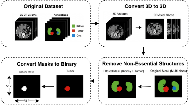
The KiTS23 kidney tumor segmentation dataset was used as the primary benchmark for analysing the effect of communication channels on deep learning segmentation of medical images. This dataset originally consisted of 3D CT volumes, along with expert-annotated masks of the kidney, tumor, and cyst regions. The applied preprocessing pipeline is summarised in Figure 3.
Figure 3. KiTS23 dataset processing pipeline
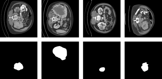
The first step involved converting the 3D volumes into 2D axial slices. This process generated 95,000 image and mask pairs. There were 6,289 image–mask pairs, excluding slices without kidney structure and excluding cyst labels. The retained annotations were converted into binary tumor–background masks, in which the tumor was assigned to the foreground and everything else to the background. There was no filtering or balancing according to tumor size or foreground proportion, and pixel-level imbalance was handled during training by implementing focal Tversky and weighted cross-entropy losses. Finally, these image samples and masks were renamed and resized to a standard spatial resolution of 512 × 512 pixels. Figure 4 demonstrates a set of images and their corresponding masks from the KiTS23 dataset.
Figure 4. KiTS23 sample images and corresponding segmentation masks
3.5 Experimental protocol
In this work, the proposed architecture HUM-Net was built using the TensorFlow and Keras deep learning environment. All experiments were conducted on the Kaggle platform equipped with dual high-end GPUs with 16 GB of memory. The KiTS23 patient cases were split into training and testing subsets at an 80:20 ratio, with patient identifiers chosen so that all patient slices were included only in one subset. Subsequently, data augmentation strategies, including flipping, rotation, and intensity variations, were applied to the training set to mitigate overfitting.
This model was systematically trained for a maximum of 100 epochs using a grid search strategy to determine the optimal hyperparameters. This resulted in a batch size of 8, an Adam optimizer, and an initial learning rate of 10⁻⁴. Moreover, the ReduceLROnPlateau technique was employed to gradually decrease the learning rate. The model was trained using a custom loss function that combines a weighted sum of focal Tversky loss and weighted cross-entropy. Early stopping was also utilised by monitoring the validation loss with a patience of 15 epochs, and the weights at the minimum point of the validation loss were saved. The convolutional kernels were initialised by He normal, and the biases were initialized by zeros. The settings were consistently applied to all models.
The computational efficiency was measured on 512 × 512 input images with a batch size of one. FLOPs were computed for a single forward pass. To measure inference latency, 20 forward passes were made after 20 warm-up iterations on the NVIDIA Tesla P100 GPU. The maximum memory consumption of the GPU was noted during the inference stage.
The models were tested with the same hardware and software configuration to ensure a fair comparison. The testing procedure was performed on 1,258 test slices, producing more than 30,000 degraded images across the 24 channel conditions. Each degraded image was processed by the trained HUM-Net to obtain a predicted segmentation mask, which was compared against the corresponding ground-truth mask using standard segmentation metrics: the DSC coefficient, mIoU, sensitivity, specificity, precision, AUC, and the 95th-percentile Hausdorff distance (HD95). The higher the value, the better for all but the metric HD95, where a lower value represents closer agreement of the boundary.
For each degraded image, four signal-quality metrics were computed against the original uncompressed reference: BER, peak signal-to-noise ratio (PSNR); structural similarity (SSIM); and CR, defined as the size of the original uint16 image divided by the size of the JPEG-encoded bitstream. BER was reported only for the noise-only and combined-stress blocks; for the compression-only block, it was set to NaN, since JPEG is a lossy intra-frame transform whose bit-level differences do not correspond to channel-induced errors. The channel- and segmentation-side metrics were merged to study the impact of the physical-layer impairments on downstream segmentation accuracy.
Additionally, training stability was evaluated by training each model five times with different random seeds. The same split and hyperparameter values were used for all runs, with weight initialisation, sample shuffling, and augmentation randomness varied between runs. The results are reported as mean ± standard deviation.
The cross-channel communication environment was simulated and applied to the kiTS23 data. The five benchmark models were evaluated using HUM-Net in both clean and degraded channel conditions.
4.1 Segmentation results
Table 2 compares five commonly used models, namely U-Net, SEG-Net, PSP-Net, FCNet, and DeepLab V2, along with the proposed model, using identical settings. Furthermore, the average and standard deviation values are reported over five independent runs in Table 2. The statistical significance of the results showed that the difference between HUM-Net and the strongest baseline was evaluated by a paired Wilcoxon signed-rank test (p < 0.05).
Table 2. Performance evaluation of segmentation models on the KiTS23 dataset over five independent runs (mean ± standard deviation)
|
Model |
mIoU |
DSC |
Precision |
Recall |
HD95 |
|
U-Net |
0.9324 ± 0.0042 |
0.9300 ± 0.0049 |
0.9139 ± 0.0049 |
0.9485 ± 0.0048 |
7.8699 ± 0.0049 |
|
SEG-Net |
0.9227 ± 0.0048 |
0.9191 ± 0.0047 |
0.9088 ± 0.0046 |
0.9296 ± 0.0050 |
8.3122 ± 0.0048 |
|
PSP-Net |
0.9267 ± 0.0049 |
0.9236 ± 0.0050 |
0.9035 ± 0.0049 |
0.9447 ± 0.0051 |
8.4548 ± 0.0044 |
|
FCNet |
0.8722 ± 0.0048 |
0.8587 ± 0.0044 |
0.8922 ± 0.0048 |
0.8276 ± 0.0041 |
11.512 ± 0.0049 |
|
DeepLab V2 |
0.9314 ± 0.0044 |
0.9288 ± 0.0052 |
0.9196 ± 0.0044 |
0.9383 ± 0.0043 |
7.9021 ± 0.0058 |
|
HUM-Net |
0.9569 ± 0.0040 |
0.9562 ± 0.0043 |
0.9561 ± 0.0047 |
0.9563 ± 0.0044 |
6.3565 ± 0.0052 |
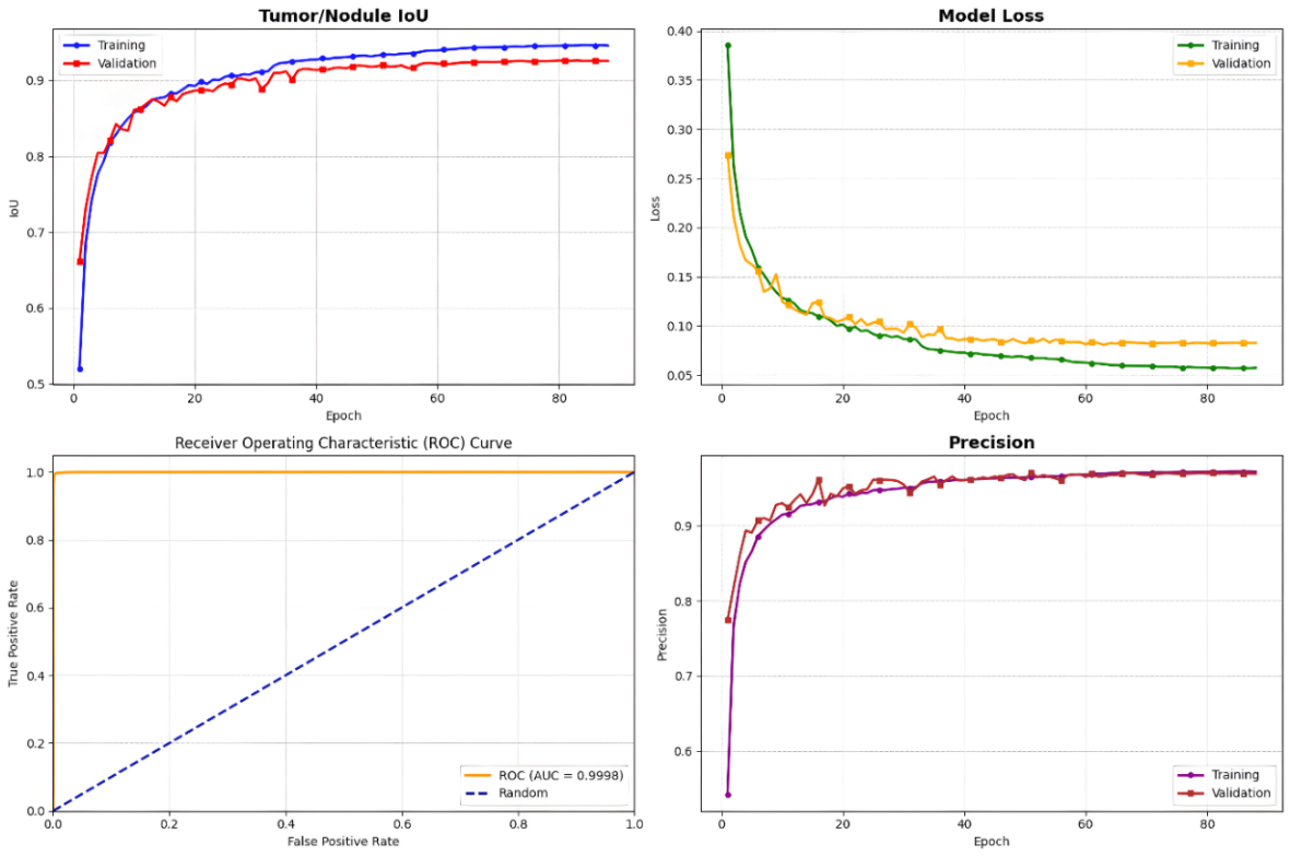
Based on the experimental results, the proposed HUM-Net framework achieved the best overall segmentation performance. Compared to the U-Net, the standard medical baseline model, which achieved an mIoU of 0.9324 and a DSC of 0.9300, HUM-Net improved the mIoU and DSC by 2.63% and 2.82%, respectively. Similarly, the proposed framework outperformed the highly complex model, DeepLab V2, by 3.97% in precision. However, these statistics only represent the model's behaviour during the evaluation and do not cover the learning behaviour of the model. Therefore, an additional set of graphs is incorporated to provide a deeper understanding of the learning dynamics with respect to the supplied inputs. The training progress in terms of the IoU, loss, ROC, and precision curves is illustrated in Figure 5.
Figure 5. Training performance curves of the proposed HUM-Net model on the KiTS23 dataset
The graphical representations in Figure 5 reflect a stable learning process, with consistent improvement during the training periods and high consistency between training and validation outcomes. Additionally, Figure 6 shows a set of qualitative samples from the KiTS23 dataset, their ground truth, the predicted segmentation using HUM-Net, and the overlaid visualisation.

Figure 6. HUM-Net segmentation results: (a) the original image, (b) the ground truth, (c) the prediction, and (d) the overlaid samples
4.1.1 Ablation study
To quantify the contribution of each architectural component, an ablation study was performed by progressively replacing each component with a baseline model comprising a residual convolutional network: (1) baseline with the VSS bottleneck, (2) baseline with SSAG, (3) baseline with both VSS and SSAG, and (4) complete HUM-Net with decoder-side state-space refinement. Further replacement experiments were conducted by replacing the VSS with a regular convolutional bottleneck and replacing SSAG with a regular attention gate, as presented in Table 3. Based on the results, considering the residual CNN baseline as a reference, VSS achieved a 0.70% increase in DSC, while SSAG achieved a larger increase of 1.21% for the same metric. The interactions of these two components led to an improvement in DSC by 1.96%, while the complete HUM-Net achieved the highest gain of 2.30%, which confirms its complementary improvements.
Table 3. Ablation study of the main components of HUM-Net
|
Model |
mIoU |
DSC |
Precision |
Recall |
|
Residual CNN Baseline |
0.9368 |
0.9346 |
0.9314 |
0.9379 |
|
Baseline + VSS |
0.9445 |
0.9431 |
0.9431 |
0.9457 |
|
Baseline + SSAG |
0.9437 |
0.9418 |
0.9440 |
0.9397 |
|
Baseline + VSS+ SSAG |
0.9538 |
0.9528 |
0.9519 |
0.9537 |
|
HUM-Net |
0.9569 |
0.9562 |
0.9561 |
0.9563 |
Note: DSC = Dice Score, VSS = Visual State Space, SSAG = State-Space Attention Gates.
4.2 Communication channel effects on HUM-Net segmentation performance
For AWGN, packet loss, JPEG compression, and combined impairments, the clean channel results were taken as the reference point.
4.2.1 Effect of the signal-to-noise ratio
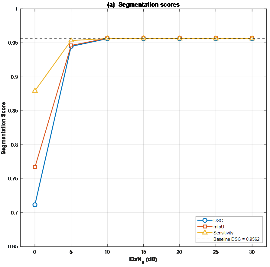
Table 4 shows that AWGN substantially affected segmentation only at very low SNR levels. At 0 dB, the mIoU index decreased by 19.8%, and similarly, the DSC decreased by 25.5%, indicating severe image distortion during transmission. Additionally, the boundaries of the regions of interest were severely affected, as evidenced by a marked increase in the HD95 metric. This performance degradation at an SNR of 0 dB can be justified by the fact that the information power becomes similar to the noise power, indicating significant distortion of the structure of medical images and thus reducing the efficiency of semantic segmentation. This negative effect gradually diminishes once the ratio is increased to 5 dB, as the segmentation performance improves significantly. Accordingly, the DSC index deterioration decreased by 1.18% compared to the baseline, indicating that the HUM-Net model has the ability to resist moderate noise levels. Subsequently, the test set was replaced with images having an SNR of 10 dB, resulting in an increase in segmentation efficiency to a near-perfect match with baseline performance. Therefore, an SNR of 10 dB can be considered the threshold beyond which added noise is insufficient to affect the semantic features extracted from medical images.
Table 4. Effect of the channel noise on medical image segmentation
|
Case |
mIoU |
DSC |
Spec. |
Sens/Recall |
HD95 |
AUC |
Precision |
|
No Effect |
0.9569 |
0.9562 |
0.9989 |
0.9563 |
6.3565 |
0.9994 |
0.9561 |
|
SNR_00 dB |
0.7669 |
0.7116 |
0.9845 |
0.8794 |
52.4025 |
0.9904 |
0.5976 |
|
SNR _05 dB |
0.9463 |
0.9449 |
0.9983 |
0.9535 |
8.4141 |
0.9992 |
0.9364 |
|
SNR _10 dB |
0.9569 |
0.9562 |
0.9988 |
0.9564 |
6.3444 |
0.9994 |
0.9560 |
|
SNR _15 dB |
0.9569 |
0.9562 |
0.9989 |
0.9563 |
6.3568 |
0.9994 |
0.9561 |
|
SNR _20 dB |
0.9569 |
0.9562 |
0.9989 |
0.9563 |
6.3568 |
0.9994 |
0.9561 |
|
SNR _25 dB |
0.9569 |
0.9562 |
0.9989 |
0.9563 |
6.3568 |
0.9994 |
0.9561 |
|
SNR _30 dB |
0.9569 |
0.9562 |
0.9989 |
0.9563 |
6.3565 |
0.9994 |
0.9561 |
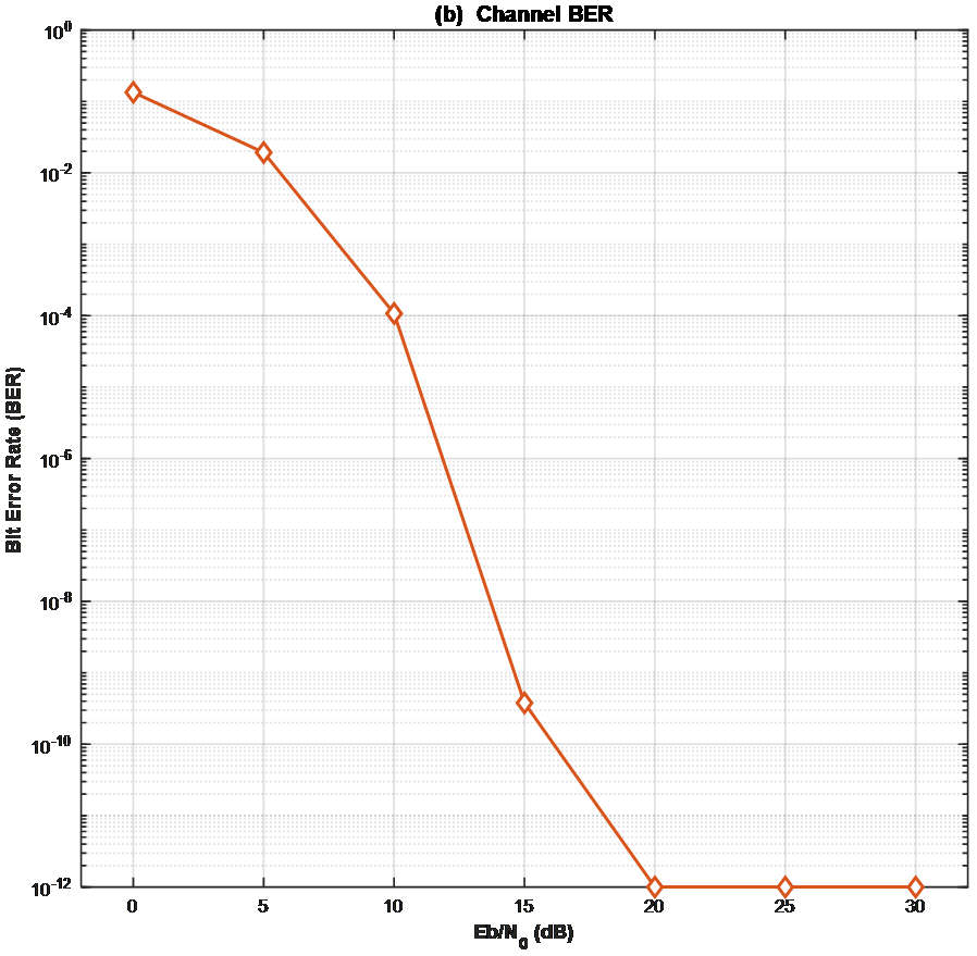
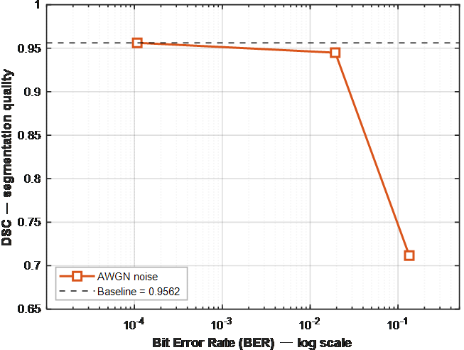
The typical behaviour of HUM-Net under AWGN is shown in Figure 7. As seen in Figure 7(a), segmentation accuracy drops steeply between 0 dB and 5 dB Eb/N0, then recovers to baseline by 10 dB and stays approximately flat thereafter. This transition occurs exactly when the BER in the channel is on the cliff, as shown in Figure 7(b), which shows the BER dropping from ~1.3 × 10⁻¹ at 0 dB to 1.1 × 10⁻⁴ at 10 dB and is effectively zero for Eb/N0 ≥ 15 dB. These results can be compared with some previous works on noise robustness of medical segmentation. When applying Gaussian noise to chest X-ray imagery, Jiu et al. [30] concluded that the DSC of DeepLab, FPN and U-Net was 0.8430, while Deb et al. [31] reported that the DSC of a conventional U-Net is acceptable under various noise types when applied to spinal stenosis imagery. Babaeipour et al. [32] noted that transformer-based segmentation models maintained high DSC and low HD95 with high noise levels, while conventional CNN models decreased more significantly. This is consistent with the latter observation, where the hybrid design is able to recover completely to baseline at or above Eb/N0 = 10 dB, while maintaining DSC = 0.9449 at Eb/N0 = 5 dB. However, there is a more fundamental question about the measurement of noise. Previous studies add noise into the image domain, usually in terms of the variance of the noise; noise levels are not easily comparable across studies and cannot be matched to a link budget. The present framework introduces noise at the waveform level and reports the Eb/N0, thus allowing the expression of robustness in the same units in which the communication system is designed. The 10 dB threshold found in the present context can thus be directly compared with the operating point of a communication system.
4.2.2 Effect of packet loss
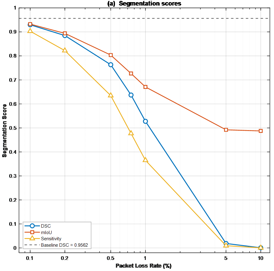
Table 5 indicates that packet loss generated more significant segmentation degradation than AWGN, as it discarded spatial contiguous image data and caused the loss of important local structural information. With a packet-loss ratio of 0.1%, the mIoU index reached 0.9326 compared to a baseline of 0.9569, showing only a limited reduction in segmentation accuracy. Similarly, the DSC index decreased by 2.76%, indicating that the HUM-Net model is capable of maintaining stable performance at low PL levels. However, increasing PL to 0.2% resulted in a significant drop in the segmentation performance for the kidney tumor. Specifically, the DSC index decreased by 7.46% compared to baseline performance, and this applies to the other metrics as well. The increased degradation suggests that higher packet loss can affect the recovery of tumor-related features and reduce the accuracy of segmentation results. At PL = 0.5%, the situation worsened as the HD95 coefficient rose negatively to 13.4980, giving the impression of a clear decrease in boundary prediction and poor segmentation in general. This result further demonstrates that severe packet loss has a stronger influence on boundary localization and overall segmentation quality.
Table 5. Effect of packet loss on medical image segmentation
|
Case |
mIoU |
DSC |
Spec. |
Sens/Recall |
HD95 |
AUC |
Precision |
|
No Effect |
0.9569 |
0.9562 |
0.9989 |
0.9563 |
6.3565 |
0.9994 |
0.9561 |
|
PL_0010 pct |
0.9326 |
0.9297 |
0.9990 |
0.9029 |
7.8699 |
0.9984 |
0.9582 |
|
PL_0020 pct |
0.8939 |
0.8848 |
0.9991 |
0.8220 |
10.0093 |
0.9956 |
0.9579 |
|
PL _0050 pct |
0.8035 |
0.7633 |
0.9993 |
0.6347 |
13.498 |
0.9849 |
0.9572 |
|
PL_0075 pct |
0.7267 |
0.6370 |
0.9995 |
0.4769 |
16.8585 |
0.9762 |
0.9590 |
|
PL_01 pct |
0.6707 |
0.5275 |
0.9995 |
0.3651 |
19.5706 |
0.9642 |
0.9497 |
|
PL_05 pct |
0.4921 |
0.0186 |
1.0000 |
0.0094 |
33.1094 |
0.8341 |
0.8778 |
|
PL_10pct |
0.4874 |
0.0007 |
1.0000 |
0.0004 |
84.4877 |
0.7781 |
0.8468 |
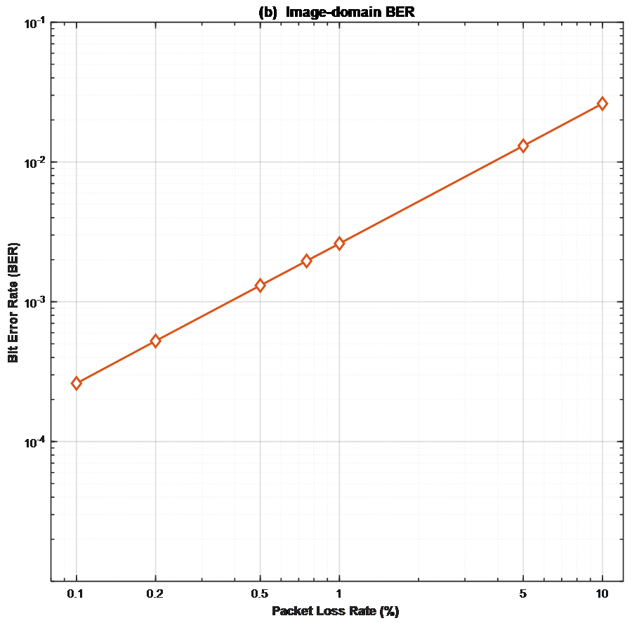
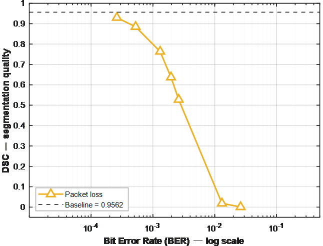
This decline continued gradually, with the most significant deterioration occurring particularly at PL with rates of 5% and 10%. At the level of 10%, the DSC score almost disappeared, reaching 0.0007, and sensitivity became virtually non-existent, indicating a complete paralysis of the segmentation system and hindering the detection of target tumor sites. Figure 8 illustrates the dominant role of packet loss in HUM-Net's degradation. A smooth, near-linear decrease in DSC is seen in the range between 0.1% and 1%, with a catastrophic decrease above 1% as seen in Figure 8(a). The DSC becomes approximately 0 at 5% and 10% loss, and sensitivity drops below 0.01, meaning that masks get very close to being empty. Figure 8(b) depicts the image-domain BER as a function of the packet-loss rate, and shows a linear behaviour as expected for the Gilbert–Elliott erasure model, which is a physically meaningful baseline for the segmentation collapse shown in Figure 8(a). In particular, packet loss rates of even a few hundredths of a percent are commonplace in 5G deployments in the medical field [4] and yield significant degradation, which is an incentive to develop explicit packet-recovery mechanisms for wireless medical imaging systems. The level of packet-loss effect seen here is significant, and should be compared to previous work. Chuprov et al. [24] concluded that packet-loss rates between 2-5% on a real wireless X-ray link reduced deep-learning performance by about 20%, while Shiranthika et al. [25] found that a split-federated U-Net was quite resilient against packet loss up to 50%, and segmentation quality dropped at higher rates. The present study, on the other hand, shows that the accuracy of segmentation is impaired even at 0.2% loss rate and rapidly goes to zero above this value. This seeming paradox is resolved by the fact that loss is applied at different points in each of the two. In Shiranthika et al. [25], the losses are incurred just at the splitting location of a federated network during the transmission of intermediate feature maps and gradients; since the networks are based on ReLU activations, the outputs are often 0, the loss value is replaced by 0 when it is lost, which provides strong intrinsic tolerance to the model. In the current setup, on the other hand, loss is applied to the transmitted picture, causing a deleted area to lose information that a subsequent computation cannot recover. The two studies therefore measure two different phenomena: feature-domain loss during collaborative training, and image-domain loss during transmission; the latter having the lower tolerance reported here is expected. The impact is compounded by two more factors. First, the tasks have different levels of sensitivity: classification combines all evidence from the entire image and can cope with corrupted evidence in local areas, while dense pixel-wise segmentation must give the correct label at each point, even if the evidence that is actually present is corrupted at that point. Second, the loss model employed here is intentionally unconcealed, since the following are deliberately discontinued: lost regions are filled with zeros and no interpolation/inpainting is performed; there is no retransmission so that each loss event corresponds directly to a loss of image content, spread out among many small blocks that are likely to overlap the edge of the tumor that determines the DSC.
The above observations indicate that the tolerance levels reported in feature-domain loss, classification, or concealment-equipped pipelines should not be applied to image-domain segmentation using pipelines without concealment, and that the operating margins for successful segmentation over lossy links may be much narrower than indicated by those studies.
4.2.3 Effect of JPEG compression
The results in Table 6 indicate that the JPEG compression had only a slight influence on segmentation. At the highest tested setting, Q = 10, the DSC metric decreased by 0.41% in the highest compression level.
Table 6. Effect of compression on medical image segmentation
|
Case |
mIoU |
DSC |
Spec. |
Sens/Recall |
HD95 |
AUC |
Precision |
|
JPEG_10 |
0.9532 |
0.9523 |
0.9988 |
0.9512 |
7.2151 |
0.9994 |
0.9534 |
|
JPEG_20 |
0.9566 |
0.9559 |
0.9988 |
0.9567 |
6.5727 |
0.9994 |
0.9550 |
|
JPEG_30 |
0.9567 |
0.956 |
0.9988 |
0.9574 |
6.4154 |
0.9994 |
0.9547 |
|
JPEG_50 |
0.9569 |
0.9562 |
0.9988 |
0.9565 |
6.3557 |
0.9994 |
0.9559 |
|
JPEG_70 |
0.9568 |
0.9561 |
0.9988 |
0.9565 |
6.2533 |
0.9994 |
0.9557 |
Similarly, the HD95 value did not increase significantly, and no noticeable changes were observed in the specificity, AUC, and precision metrics despite the high compression level. However, increasing the compression level to 70 resulted in a negligible effect, and the metric values remained consistent with baseline conditions. This performance stability can be explained by the fact that changing the compression level masks high-frequency information, which is less important in semantic segmentation, a process that relies primarily on structural patterns and semantic context.
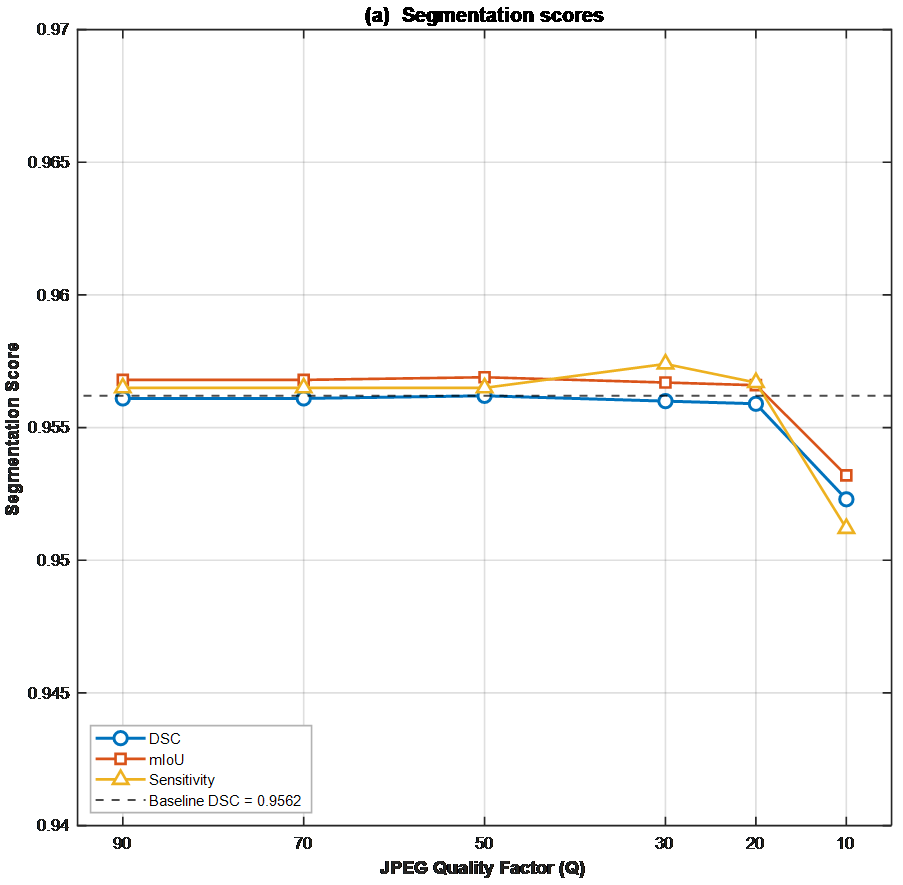
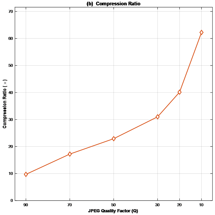
Figure 9 shows that HUM-Net is extremely resistant to lossy source coding. Note that even at the highest tested JPEG aggressiveness (Q = 10), DSC is within 0.4% of baseline (0.9523 vs. 0.9562), as seen in Figure 9(a). The mIoU and sensitivity curves are also flat in all the Q = 10-90 range. The compression ratio is plotted as a function of Q in Figure 9(b), increasing from ~10× at Q = 90 to >56× at Q = 10. The addition of stable segmentation accuracy and high bandwidth reduction indicates that HUM-Net can be used without retraining or specialised preprocessing for aggressive JPEG compression to reduce the transmission load in wireless medical imaging. These results can be compared with those of previous compression results. Chen et al. [27] reported that digital-pathology images could be compressed by 85% while retaining about 95% of downstream deep-learning performance, and Neena and Anil Kumar [29] reported that classification accuracy in MRI was preserved at a 6:1 ratio, but dropped significantly at a 25:1 ratio. El Khoury et al. [28] reported promising results for a 2D U-Net on pelvic CT with a DSC of 0.7 at 50% compression. The present results add to this picture: at Q = 10 (or compression ratio = 56:1), HUM-Net still has a DSC of 0.9523 compared to a baseline of 0.9562, a 0.4% reduction. The tolerance that was observed here is therefore much higher than the previously reported tolerances. A possible reason could be that JPEG quantization sorts out the high-frequency details, while low-frequency intensity variations are more important for delineating the large, high-contrast kidney and tumor regions targeted in this study. Tasks requiring fine texture, like the histopathology and classification tasks noted in the above studies, would be expected to deteriorate earlier, and this is consistent with the lower thresholds reported in these studies.
4.2.4 The combined effect of PL and signal-to-noise ratios
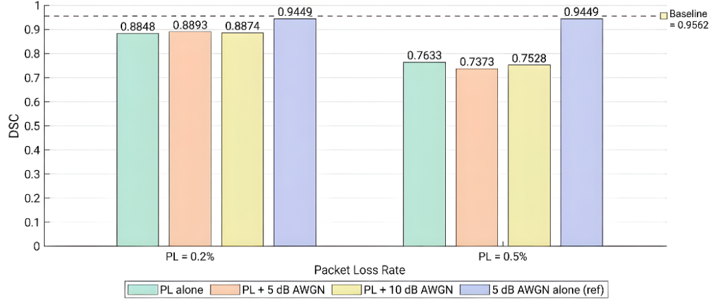
Table 7 compares the combined effects of packet loss and AWGN. At PL = 0.2% and SNR = 5 dB, mIoU and DSC decreased to 0.8976 and 0.8893, respectively, while the HD95 metric increased to 10.5129. Notably, these values are essentially identical to the PL = 0.2% standalone case (DSC = 0.8848), indicating that packet loss, and not the added 5 dB channel noise, is the dominant impairment in this regime. Similarly, increasing the SNR level from 5 to 10 dB while keeping the PL level constant resulted in only a slight change (DSC = 0.8874), confirming that once a non-trivial PL rate is present, additional channel-noise mitigation yields diminishing returns. In the same manner, the test set was evaluated using the proposed model with a PL of 0.5% and an SNR of 5 dB. This combination resulted in a sharp decline in performance, with the DSC score dropping by 22.8% compared to the baseline and the sensitivity decreasing to 0.6055, indicating an inaccurate prediction of the anatomical structures in the kidney images. Importantly, this DSC (0.7373) again tracks the PL = 0.5% standalone value (0.7633) far more closely than the SNR = 5 dB standalone value (0.9449), reinforcing the dominance of packet loss over channel noise under combined stress.
Table 7. Combined effect of packet loss and channel noise (AWGN) on medical image segmentation.
|
Case |
mIoU |
DSC |
Spec. |
Sens/Recall |
HD95 |
AUC |
Precision |
|
Combined_PL_0020bp_SNR_05dB |
0.8976 |
0.8893 |
0.9987 |
0.8395 |
10.5129 |
0.9940 |
0.9454 |
|
Combined_PL_0020bp_SNR_10dB |
0.8961 |
0.8874 |
0.9990 |
0.8271 |
9.81740 |
0.9955 |
0.9572 |
|
Combined_PL_0050bp_SNR_05dB |
0.7864 |
0.7373 |
0.9990 |
0.6055 |
14.7890 |
0.9733 |
0.9425 |
|
Combined_PL_0050bp_SNR_10dB |
0.7965 |
0.7528 |
0.9993 |
0.6209 |
14.2927 |
0.9861 |
0.9559 |
Finally, the SNR was increased to 10 dB while maintaining the PL level at 0.5%. This scenario yielded a slight improvement compared to the previous case, where HD95 decreased from 14.7890 to 14.2927. In both cases, the segmentation quality remained low compared to the baseline situation. In summary, the combined effect does not amplify the impact of either impairment beyond what is observed in isolation. Instead, the resulting DSC scores track the packet-loss-only curve much more closely than the noise-only curve (a ±2.6% DSC difference across all four combined conditions), establishing packet loss as the dominant degradation factor under realistic combined transmission stress. This highlights the critical need for reliable packet-recovery mechanisms in terms of channel coding, retransmission, or application-layer interleaving in communication-based medical imaging systems. The hierarchy of dominance is quantified in Figure 10. The three left-most bars (PL alone, PL + 5 dB AWGN, PL + 10 dB AWGN) are almost identical, while the right-most bar (5 dB AWGN alone) is significantly higher. Similarly, it is the case that channel-side noise mitigation is not sufficient to achieve HUM-Net's baseline performance unless packet erasures are first solved. It is the main practical result of the wireless-robustness study.
Figure 10. Combined-stress dominance: grouped comparison of Dice Score (DSC) at PL = 0.2% and PL = 0.5%, each evaluated alone, combined with 5 dB AWGN, combined with 10 dB AWGN, and compared against 5 dB AWGN alone (reference)
4.2.5 Baseline comparison under channel degradation
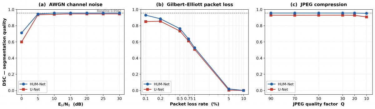
Figure 11 compares HUM-Net and U-Net with the same degraded images to see if the observed hierarchy of impairments is architecture-specific. The results demonstrate the same pattern of impairments for both models. For AWGN noise (Figure 11(a)), both recover from a low-SNR minimum to a high-SNR plateau and show a sharp transition at about 5 dB for both. In both cases, both fall off smoothly into the sub-percent domain and are close to zero when packet loss is larger than 1% (Figure 11(b)). With JPEG compression (Figure 11(c)), both are near their clean baselines over the range of quality. Thus, the ordering of the severity of the impairment is reproduced by U-Net, which indicates that it is a property of the wireless channel and segmentation problem, but not of the HUM-Net architecture.
Figure 11. Baseline comparison of HUM-Net and U-Net under channel degradation: (a) AWGN channel noise, (b) Gilbert–Elliott packet loss, and (c) JPEG compression. Both models follow the same impairment hierarchy, while HUM-Net retains a consistent advantage across all conditions
Meanwhile, HUM-Net maintains its consistent performance gain over U-Net at all the conditions explored. The advantage is at its minimum when the stress applied to both models is minimal, in the noise plateau and throughout the compression range, where both models are operating near baseline (the DSC margin of ~0.011 and ~0.026 respectively), but the advantage is largest under the most severe stress: at 0 dB, the margin between HUM-Net and U-Net is 0.112 DSC, and at the onset of packet loss, the difference is 0.080 DSC. This means that the hybrid state-space design is optimal in the most degraded channel, the place where robustness is most needed, and neither of the designs is immune to the fundamental problem of packet loss. The implication that follows in the next subsections, which is that packet-loss recovery should be a design priority, does not restrict the segmentation model to the architecture proposed here but is, rather, a general one for any system.
4.3 Cross-domain quality analysis
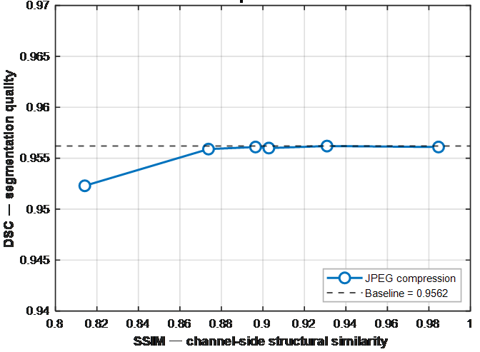
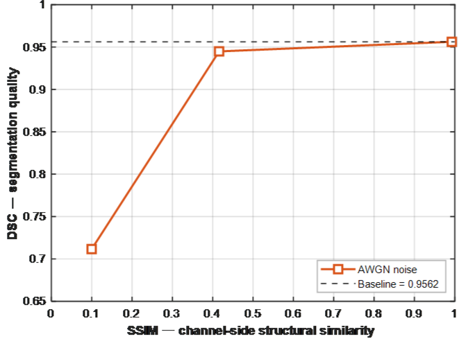
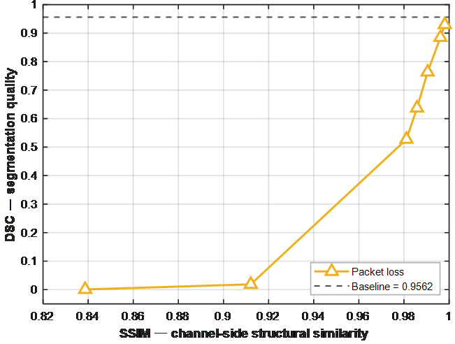
For every condition, a physical-layer metric (PSNR, SSIM, or BER) was paired with the HUM-Net DSC to see if conventional channel-quality measures can predict the segmentation accuracy. The channel quality-segmentation accuracy relationship is strongly dependent on the impairment type, as illustrated in Figure 12. As can be seen in panel (a), even as PSNR decreases to 26 dB, DSC is retained at 0.95. At the same PSNR, however, noise produces a steep DSC drop (panel b), whereas packet loss in panel (c) yields a markedly different DSC, confirming that identical PSNR values map to very different segmentation outcomes depending on the impairment type. The lesson learned is that channel-quality metrics need to be combined with impairment-type information to predict the outcomes of segmentation, which is beyond PSNR.
The most direct relationship between physical-layer error rates and segmentation outcomes is available in Figure 13. For AWGN (panel a), DSC recovers to baseline as the channel BER falls from 1.3 × 10⁻¹ to 1 × 10⁻⁴, as expected from the textbook QPSK curve. But under packet loss (panel b), the same BER range corresponds to a much larger DSC range, ranging from 0.93 to almost zero, which shows that BER alone is not sufficient to determine the quality of segmentation. These curves can be directly linked from achieved channel BER to expected segmentation accuracy and provide an initial quantitative reference for the choice of modulation, coding and packet-recovery schemes in wireless medical imaging links, subject to validation on deployed links.
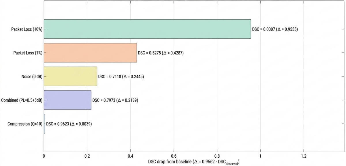
The correlation between the metrics collected on the channel side and the accuracy of the segmentation has not been described before, to the best of our knowledge. The medical-imaging studies presented in Section 2 report task performance under individual impairments; in earlier work, it was shown that image-quality degradation impacts the performance of deep classifiers; however, none of these studies correlate measures of physical-layer impairments, like bit error rate, or reconstruction impairments, like PSNR and SSIM, with the quality of segmentation downstream. The present results show that PSNR, SSIM and BER are not reliable measures of segmentation reliability, because the same channel-side value can correspond to very different DSC depending on the type of impairment, most strikingly between compression and erasure, which yield similar PSNR or SSIM yet very different segmentation quality. This also suggests that there is a need for segmentation-aware quality-of-service indicators, as discussed in Section 5. Figure 14 summarises the wireless-robustness study in a single visual. The Figure is the main message of this work: Design effort should focus on packet-loss recovery rather than compression mitigation or channel-noise reduction, both of which HUM-Net tolerates across the ranges examined.
4.4 Assumptions and limitations
The framework is an abstraction of a deployed wireless link; the boundaries of the framework should be explicitly stated. The channel is assumed to be AWGN and thus does not consider multipath fading, Doppler, and shadowing. No coding, no forward error correction or hybrid ARQ and retransmission, and no adaptive modulation and coding are used. Co-channel interference, scheduling and handover dynamics are not considered; it is a single-user link. Apart from the compensation for the cascaded filter group delay, this is idealised synchronisation without any induction of carrier frequency offset, carrier phase noise and timing jitter. The transport and application protocol stack is not modelled, nor is latency. Finally, the packet loss and noise processes are independent processes, compared to a real link where they are both influenced by the same channel state. The nature of these simplifications varies. The degradation reported does not account for the protection provided by channel coding and retransmission, and would be significantly lower in a coded system at a given raw SNR. If fading is not included, on the other hand, it is optimistic as compared to a mobile channel with deep fades. The framework is therefore designed to be applied to a segmentation model, with controlled and repeatable impairments, and is not designed to predict the end-to-end performance of a specific deployed network. The evaluation was simulation-only, as no measurement was taken on real communication devices and end-to-end latency, one of the key factors in interactive telemedicine, was not modelled. The cost of inference was not profiled on the edge or embedded hardware that would be used with such deployments. Lastly, segmentation accuracy was compared with reference annotations on a single public dataset, and clinical validation was not performed; whether the observed accuracy decreases lead to a diagnostic error, and what constitutes an acceptable threshold, remains to be determined and would require reader studies with clinical endpoints. These results should thus be interpreted as describing the inherent sensitivity of a segmentation model to common channel impairments, and as an impetus for deployment-level and clinical testing rather than a replacement for such testing. A natural extension is to incorporate a full JPEG2000 codestream packetization layer with DICOM transport syntax and standardised error concealment, which would refine the present conservative bounds into codec-specific operating curves.
In this work, we proposed HUM-Net, a lightweight U-Mamba segmentation architecture, and a physically grounded end-to-end simulation framework for robust assessment of deep medical image segmentation under realistic wireless channel impairments. The proposed architecture, along with the proposed evaluation framework, together offer a consistent way of assessing not only the performance of a segmentation model with clean data, but also its performance degradation with the same data received via a JPEG-encoded and noisy wireless link that is lossy. On the KiTS23 test set with 1,258 slices, the baseline performance of HUM-Net was: DSC coefficient of 0.9562, HD95 of 6.36, and mIoU of 0.9569, which were better than the U-Net baseline, SEG-Net baseline, FCNet baseline, PSP-Net baseline, and DeepLab V2 baseline. The wireless-robustness study showed that across 24 different channel conditions covering over 30,000 degraded images, there is a definite order of impairments from worst to best. The DSC score for HUM-Net was not noticeably affected by lossy JPEG compression, even at a value of Q = 10 (compression ratio 56×). Channels with noise levels above 10 dB Eb/N₀ were completely recoverable, while for high noise levels (around 0 dB Eb/N₀), the DSC went down to 0.7116 with a sharp transition around 5 dB. In contrast, the most disruptive impairment was packet loss, and as packet loss increased, the DSC dropped to 0.8848 at 0.2%, and dropped close to zero when the packet loss rate was above 1% segmentation accuracy. For the combined-stress block, packet loss always dominated channel noise; the combined DSC scores followed the packet-loss-only curve much more closely than the noise-only curve, and the interaction between the two impairments was only mild (±2.6% DSC). Importantly, the cross-domain analysis also revealed that traditional metrics of channel quality (PSNR, SSIM, and BER) are not good indicators of the segmentation accuracy: packet loss in particular results in significant segmentation collapse at PSNR and SSIM values that would be considered acceptable. These findings collectively suggest design priorities for wireless medical imaging systems. The results suggest that HUM-Net may tolerate modest link margins and aggressive bandwidth reduction without retraining or specialized pre-processing for lossy compression and moderate channel noise. However, channel coding, retransmission, or application-layer interleaving are indicated as countermeasures warranting investigation, even at rates of packet loss that are relatively small, say in the sub-percent range. The results highlight the need for further research into segmentation-aware quality-of-service metrics to reflect the operational effect of physical-layer impairments on downstream clinical activities in future work.
[1] Heller, N., Isensee, F., Maier-Hein, K.H., et al. (2021). The state of the art in kidney and kidney tumor segmentation in contrast-enhanced CT imaging: Results of the KiTS19 challenge. Medical Image Analysis, 67: 101821. https://doi.org/10.1016/j.media.2020.101821
[2] Bilic, P., Christ, P., Li, H.B., et al. (2023). The liver tumor segmentation benchmark (LITS). Medical Image Analysis, 84: 102680. https://doi.org/10.1016/j.media.2022.102680
[3] Menze, B.H., Jakab, A., Bauer, S., et al. (2014). The multimodal brain tumor image segmentation benchmark (BRATS). IEEE Transactions on Medical Imaging, 34(10): 1993-2024. https://doi.org/10.1109/TMI.2014.2377694
[4] Soldani, D., Fadini, F., Rasanen, H., et al. (2017). 5G mobile systems for healthcare. In 2017 IEEE 85th Vehicular Technology Conference (VTC Spring), Sydney, Australia, pp. 1-5. https://doi.org/10.1109/VTCSpring.2017.8108602
[5] Chen, M., Hao, Y., Hwang, K., Wang, L., Wang, L. (2017). Disease prediction by machine learning over big data from healthcare communities. IEEE Access, 5: 8869-8879. https://doi.org/10.1109/ACCESS.2017.2694446
[6] Ronneberger, O., Fischer, P., Brox, T. (2015). U-net: Convolutional networks for biomedical image segmentation. In International Conference on Medical Image Computing and Computer-Assisted Intervention, pp. 234-241. https://doi.org/10.1007/978-3-319-24574-4_28
[7] Cao, H., Wang, Y., Chen, J., et al. (2022). Swin-unet: Unet-like pure transformer for medical image segmentation. In European Conference on Computer Vision, pp. 205-218. https://doi.org/10.1007/978-3-031-25066-8_9
[8] Chen, J., Mei, J., Li, X., et al. (2024). TransUNet: Rethinking the U-Net architecture design for medical image segmentation through the lens of transformers. Medical Image Analysis, 97: 103280. https://doi.org/10.1016/j.media.2024.103280
[9] Gu, A., Dao, T. (2023). Mamba: Linear-time sequence modeling with selective state spaces. arXiv preprint arXiv:2312.00752. https://doi.org/10.48550/arXiv.2312.00752
[10] Liu, Y., Tian, Y., Zhao, Y., et al. (2024). Vmamba: Visual state space model. Advances in neural Information Processing Systems, 37: 103031-103063. https://doi.org/10.52202/079017-3273
[11] Ma, J., Li, F., Wang, B. (2024). U-mamba: Enhancing long-range dependency for biomedical image segmentation. arXiv preprint arXiv:2401.04722. https://doi.org/10.48550/arXiv.2401.04722
[12] Abdani, S.R., Zulkifley, M.A., Zulkifley, N.H. (2021). Group and shuffle convolutional neural networks with pyramid pooling module for automated pterygium segmentation. Diagnostics, 11(6): 1104. https://doi.org/10.3390/diagnostics11061104
[13] Zulkifley, M.A. (2026). Automated segmentation of pterygium lesions using multiscale deep learning networks. Experimental Eye Research, 266: 110928. https://doi.org/10.1016/j.exer.2026.110928
[14] Dodge, S., Karam, L. (2016). Understanding how image quality affects deep neural networks. In 2016 Eighth International Conference on Quality of Multimedia Experience (QoMEX), Lisbon, Portugal, pp. 1-6. https://doi.org/10.1109/QoMEX.2016.7498955
[15] Feng, Y., Cai, Y. (2020). Towards robust classification with image quality assessment. arXiv preprint arXiv:2004.06288. https://doi.org/10.48550/arXiv.2004.06288
[16] Hendrycks, D., Dietterich, T. (2019). Benchmarking neural network robustness to common corruptions and perturbations. arXiv preprint arXiv:1903.12261. https://doi.org/10.48550/arXiv.1903.12261
[17] Ghoben, M.K., Muhammed, L.A.N. (2023). Exploring the impact of image quality on convolutional neural networks: A study on noise, blur, and contrast. In 2023 International Conference of Computer Science and Information Technology (ICOSNIKOM), Binjia, Indonesia, pp. 1-7. https://doi.org/10.1109/ICoSNIKOM60230.2023.10364394
[18] Karimi, D., Warfield, S.K., Gholipour, A. (2021). Transfer learning in medical image segmentation: New insights from analysis of the dynamics of model parameters and learned representations. Artificial Intelligence in Medicine, 116: 102078. https://doi.org/10.1016/j.artmed.2021.102078
[19] Zedan, M.J., Abdani, S.R., Lee, J., Zulkifley, M.A. (2025). RMHA-Net: robust optic disc and optic cup segmentation based on residual multiscale feature extraction with hybrid attention networks. IEEE Access, 13: 7715-7735. https://doi.org/10.1109/ACCESS.2025.3525813
[20] Elizar, E., Muharar, R., Zulkifley, M.A. (2024). DeSPPNet: A multiscale deep learning model for cardiac segmentation. Diagnostics, 14(24): 2820. https://doi.org/10.3390/diagnostics14242820
[21] Abdani, S.R., Zulkifley, M.A., Zulkifley, N.H. (2021). Group and shuffle convolutions for high-resolution semantic segmentation. In 2021 International Conference on Decision Aid Sciences and Application (DASA), Sakheer, Bahrain, pp. 12-16. https://doi.org/10.1109/DASA53625.2021.9682288
[22] Ruan, J., Li, J., Xiang, S. (2024). Vm-UNet: Vision Mamba UNet for medical image segmentation. ACM Transactions on Multimedia Computing, Communications and Applications. https://doi.org/10.1145/3767748
[23] Liu, J., Yang, H., Zhou, H.Y., et al. (2024). Swin-umamba: Mamba-based UNet with ImageNet-based pretraining. In International Conference on Medical Image Computing and Computer-Assisted Intervention, pp. 615-625. https://doi.org/10.1007/978-3-031-72114-4_59
[24] Chuprov, S., Satam, A.N., Reznik, L. (2022). Are ML image classifiers robust to medical image quality degradation? In 2022 IEEE Western New York Image and Signal Processing Workshop (WNYISPW), Rochester, USA, pp. 1-4. https://doi.org/10.1109/WNYISPW57858.2022.9983488
[25] Shiranthika, C., Kafshgari, Z.H., Saeedi, P., Bajić, I.V. (2023). SplitFed resilience to packet loss: Where to split, that is the question. In International Conference on Medical Image Computing and Computer-Assisted Intervention, pp. 367-377. https://doi.org/10.1007/978-3-031-47401-9_35
[26] Rashmi, P., Gomathi, R. (2024). Optimized deep learning frameworks for the medical image transmission in IoMT environment. Journal of Smart Internet of Things, 2024(2): 148-165. https://doi.org/10.2478/jsiot-2024-0018
[27] Chen, Y., Janowczyk, A., Madabhushi, A. (2020). Quantitative assessment of the effects of compression on deep learning in digital pathology image analysis. JCO Clinical Cancer Informatics, 4: 221-233. https://doi.org/10.1200/CCI.19.00068
[28] El Khoury, K., Fockedey, M., Brion, E., Macq, B. (2021). Improved 3D U-Net robustness against JPEG 2000 compression for male pelvic organ segmentation in radiotherapy. Journal of Medical Imaging, 8(4): 041207-041207. https://doi.org/10.1117/1.JMI.8.4.041207
[29] Neena, K.A., Anil Kumar, M.N. (2026). Optimizing medical MRI brain image classification through compression analysis on deep learning models with light weight implementation. International Journal of Computer Theory and Engineering, 18(1): 68-78. https://doi.org/10.7763/IJCTE.2026.V18.1389
[30] Jiu, D., Nijjer, K., Chinta, N., Bui, R., Zhu, K. (2025). Evaluating the impact of radiographic noise on chest X-ray semantic segmentation and disease classification using a scalable noise injection framework. arXiv preprint arXiv:2509.25265. https://doi.org/10.48550/arXiv.2509.25265
[31] Deb, M., Matthews, A.A., Sam, D., Jesalba, J. (2023). Effects of noise on neural network based semantic segmentation of lumbar MRI for stenosis boundary delineation. AIP Conference Proceedings, 2790(1): 020015. https://doi.org/10.1063/5.0153823
[32] Babaeipour, R., Fox, M.S., Parraga, G., Ouriadov, A. (2025). Robust segmentation of lung proton and hyperpolarized gas MRI with vision transformers and CNNs: A comparative analysis of performance under artificial noise. Bioengineering, 12(8): 808. https://doi.org/10.3390/bioengineering12080808
[33] Li, A., Liu, X., Wang, G., Zhang, P. (2022). Domain knowledge driven semantic communication for image transmission over wireless channels. IEEE Wireless Communications Letters, 12(1): 55-59. https://doi.org/10.1109/LWC.2022.3216994
[34] Yuan, W., Ren, J., Wang, C., et al. (2025). Generative semantic communication for joint image transmission and segmentation. In 2025 IEEE International Conference on Communications Workshops (ICC Workshops), Montreal, Canada, pp. 1110-1115. https://doi.org/10.1109/ICCWorkshops67674.2025.11162317
[35] Guo, F., Zheng, H., Zhang, X., Chen, L., Wang, Y., Zhang, S. (2025). DiSC-Med: Diffusion-based semantic communications for robust medical image transmission. In GLOBECOM 2025-2025 IEEE Global Communications Conference, Taipei, China, pp. 6358-6363. https://doi.org/10.1109/GLOBECOM59602.2025.11432041
[36] Badrinarayanan, V., Kendall, A., Cipolla, R. (2017). Segnet: A deep convolutional encoder-decoder architecture for image segmentation. IEEE Transactions on Pattern Analysis and Machine Intelligence, 39(12): 2481-2495. https://doi.org/10.1109/TPAMI.2016.2644615
[37] Long, J., Shelhamer, E., Darrell, T. (2015). Fully convolutional networks for semantic segmentation. IEEE Transactions on Pattern Analysis and Machine Intelligence, 39(4): 640-651. https://doi.org/10.1109/TPAMI.2016.2572683
[38] Zhao, H.S., Shi, J.P., Qi, X.J., Wang, X.G., Jia, J.Y. (2017). Pyramid scene parsing network. In 2017 IEEE Conference on Computer Vision and Pattern Recognition (CVPR), Honolulu, USA, pp. 6230-6239. https://doi.org/10.1109/CVPR.2017.660
[39] Chen, L.C., Papandreou, G., Kokkinos, I., Murphy, K., Yuille, A.L. (2017). Deeplab: Semantic image segmentation with deep convolutional nets, atrous convolution, and fully connected CRFS. IEEE Transactions on Pattern Analysis and Machine Intelligence, 40(4): 834-848. https://doi.org/10.1109/TPAMI.2017.2699184