Nur Qudus* | Rizky Ajie Aprilianto | Harianingsih Harianingsih | Bambang Sugiyarto | Virgiawan Adi Kristianto | Nur Anita | Jurina Jaafar | Eeydzah Aminudin | Noor Sahidah Samsudin | Abdrabbi Bourezg | Abdelbasset Azzouz | Rizki Mendung Ariefianto | Asad Ali Chandio
© 2026 The authors. This article is published by IIETA and is licensed under the CC BY 4.0 license (http://creativecommons.org/licenses/by/4.0/).
OPEN ACCESS
Cooling demand is a major component of building energy use in tropical climates. However, estimating it during the early design stage remains difficult because courtyard geometry and envelope characteristics interact in nonlinear ways. This study optimizes the hyperparameters of a Multi-Layer Perceptron (MLP) model for cooling load prediction using five metaheuristic algorithms: Genetic Algorithm (GA), Differential Evolution (DE), Particle Swarm Optimization (PSO), Grey Wolf Optimizer (GWO), and Harris Hawks Optimization (HHO), applied to three courtyard building configurations (L-shape, O-shape, U-shape) in Shah Alam, Malaysia. The analysis used 8,535 samples generated through parametric IES Virtual Environment (IESVE) simulations. Each algorithm was run five times, and model performance was examined using seven statistical metrics together with a Friedman test. Across the reported runs, GWO produced the highest mean test-set accuracy (R² = 0.5836; RMSE = 0.8106 kWh/m²), whereas DE showed the smallest run-to-run variation in R² (standard deviation = 0.0024). The Friedman test indicated differences in algorithm rankings (statistics = 13.44, p = 0.0093), although the five-run design limited the power of pairwise post-hoc comparisons. Permutation importance identified window-to-wall ratio as the dominant predictor within the available feature set. Per-shape evaluation showed very high accuracy for the L- and U-shaped configurations but substantially weaker performance for the fully enclosed O-shape, where repeated predictor combinations were associated with different cooling-load values. The results therefore support the use of metaheuristic-tuned MLP models as an early-stage screening surrogate for open courtyard configurations, while also highlighting the need for additional geometric, envelope, and climate-related predictors before the approach is extended to enclosed courtyard forms.
cooling load prediction, metaheuristic optimization, Multi-Layer Perceptron, courtyard buildings, tropical climate, building energy efficiency
The building sector is one of the largest consumers of energy worldwide, accounting for approximately 40% of total primary energy consumption in many developed and developing nations [1]. In tropical climates, this issue is particularly pressing because cooling systems operate year-round due to persistently high ambient temperatures and humidity [2]. The increasing urbanization of Southeast Asian cities, including those in Malaysia and Indonesia, has accelerated the construction of buildings, many of which incorporate traditional courtyard configurations as passive design strategies [3]. Courtyards are well established as architectural elements that moderate indoor thermal conditions by promoting natural ventilation, shading, and daylighting [4]. However, the relationship between courtyard morphology and building energy performance is complex and nonlinear, making accurate cooling-load prediction challenging at the early design stage.
Conventional methods for estimating cooling load rely on detailed energy simulation software such as EnergyPlus, DesignBuilder, and IES Virtual Environment (IESVE) [5]. These tools require complete specification of building geometry, envelope properties, and occupancy schedules, which are rarely available during the conceptual design phase [6]. As a result, energy performance is often evaluated only after major design decisions have been finalized, limiting opportunities to implement effective passive cooling strategies. The disconnection between energy assessment and early-stage design has been widely recognized as a critical barrier to building energy efficiency improvement [7].
Machine-learning models offer a useful surrogate for this early-stage problem because they can learn nonlinear relationships between a limited set of design variables and energy outcomes. Artificial neural networks (ANNs), support vector regression (SVR), random forests (RF), and decision trees (DT) have all been applied to building-energy prediction [8]. Among these, the Multi-Layer Perceptron (MLP) is widely applied due to its universal approximation capability and suitability for capturing nonlinear relationships between input features and energy outputs. However, MLP predictive performance is sensitive to hyperparameter selection, including the number of neurons per hidden layer, the regularization coefficient, and the learning rate. Suboptimal hyperparameter settings can lead to underfitting or overfitting, reducing the reliability of predictions [9].
Metaheuristic optimization provides one way to search for this hyperparameter space without relying on gradient information [10]. These algorithms are population-based or trajectory-based search methods that explore the solution space without requiring gradient information, making them suitable for optimizing non-differentiable and multimodal objective functions [11]. Several studies have integrated mathematical algorithms with ANN or MLP models for building energy prediction. Zheng et al. [12] applied a shuffled complex evolution algorithm to optimize an MLP for cooling load prediction and reported improvements in learning and prediction accuracy exceeding 19% compared to a standard MLP. Afzal et al. [13] compared multiple metaheuristic optimizers including Satin Bowerbird Optimizer, Ant Lion Optimizer, Slime Mold Optimizer, and Particle Swarm Optimization (PSO) for predicting heating and cooling loads using SVR and extreme gradient boosting. Mu et al. [14] demonstrated that metaheuristic-optimized MLP models trained with systematic data preprocessing achieved lower prediction errors compared to models without preprocessing, highlighting the importance of both algorithm selection and data quality. Despite these advances, the literature has not reported a comparative assessment of multiple algorithmically diverse methods applied to courtyard building typologies in tropical climates.
This study addresses this gap by evaluating five metaheuristic algorithms from the evolutionary and swarm-based optimization categories to optimize MLP hyperparameters for cooling-load prediction. This study investigates three courtyard building shapes: L-shape, O-shape, and U-shape. These configurations represent common courtyard typologies found in tropical regions and differ in enclosure degree, spatial geometry, and exposure to solar radiation. The dataset was generated from parametric energy simulations conducted in IESVE, covering 8,535 combinations of building morphology and envelope variables. The objective function used during optimization is the mean cross-validated RMSE on the training set, ensuring that the selected hyperparameters generalize well to unseen data. Each optimized model evaluated on an independent test set using seven statistical metrics, and the statistical significance of differences between algorithms was assessed using the Friedman test across multiple independent runs.
The main contributions of this study are as follows:
(1) This work provides a comparative assessment of five metaheuristic search strategies for tuning an MLP-based cooling-load predictor for tropical courtyard buildings under a common experimental framework.
(2) This work evaluates optimizer behavior using multiple performance measures, convergence information, and repeated stochastic runs rather than relying on a single optimization run.
(3) This examines the influence of courtyard form in a tropical context and identifies an important limitation in the fully enclosed O-shaped subset, thereby clarifying where the proposed surrogate is currently most dependable and where additional design variables are needed.
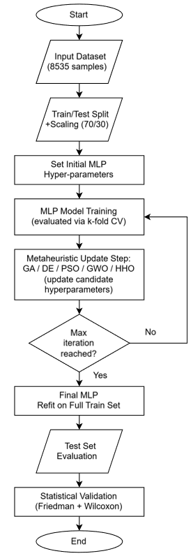
The methodology of this study consists of four main components: (a) data preparation and description of the study context; (b) description of the MLP model and its hyperparameter search space; (c) description of the five metaheuristic algorithms used for optimization; and (d) performance evaluation framework. Figure 1 presents the study’s overall workflow.
Figure 1. The workflow of this study
2.1 Study context and dataset
The dataset was generated from parametric energy simulations of courtyard buildings located in Shah Alam, Selangor, Malaysia (3.07°N, 101.52°E) [15]. Shah Alam has a tropical rainforest climate, with year-round temperatures of approximately 23–35 ℃, high relative humidity, and no pronounced dry season. Under these conditions, cooling demand is a central component of building-energy performance and is therefore used as the target outcome in this study.
This study investigated three courtyard building shapes: L-shape, O-shape, and U-shape. These typologies were selected because they represent the most common configurations of courtyard residential buildings in the region and differ substantially in terms of enclosure ratio, self-shading potential, and courtyard microclimate. Energy simulations were conducted using IESVE software, which has been validated for tropical building energy modeling. A total of 8,535 simulation samples were generated across the three configurations, comprising 1,536 samples for L-shape, 5,463 for O-shape, and 1,536 for U-shape. The dataset is therefore imbalanced across courtyard shape, with O-shape accounting for approximately 64% of all samples.
Eight input variables were considered, representing key aspects of building morphology and envelope design. These variables are building width (WIDTH), building length (LENGTH), building height (HEIGHT), building orientation (ORIENTATION), window-to-wall ratio (WINDOWS_RATIO), form factor (FORM_FACTOR), surface-to-volume ratio (S_V_RATIO), and courtyard shape encoded as a categorical variable (SHAPE). Table 1 summarizes the input variables and their respective ranges. The target variable is the annual cooling load intensity expressed in kWh/m².
Table 1. Input variables and their ranges used in the parametric simulation dataset
|
Variable |
Description |
Range |
|
WIDTH |
Building width (m) |
30.00–60.00 |
|
LENGTH |
Building length (m) |
30.00–60.00 |
|
HEIGHT |
Building height (m) |
8.00–16.00 |
|
ORIENTATION |
Building orientation (degrees) |
0.00–315.00 |
|
WINDOWS_RATIO |
Window-to-wall ratio |
0.10–0.40 |
|
FORM_FACTOR |
Building form factor |
0.77–1.89 |
|
S_V_RATIO |
Surface-to-volume ratio (m-1) |
0.19–0.47 |
|
SHAPE |
Courtyard building shape |
Categorical: L, U, O |
Prior to model training, building orientation was encoded using sine and cosine transformations to preserve its cyclical nature. The categorical shape variable was encoded using one-hot encoding, producing three binary indicator variables corresponding to L-shape, O-shape, and U-shape. All continuous input features were subsequently normalized to the range [0, 1] using Min-Max scaling, with the scaling parameters fitted exclusively on the training set to prevent data leakage.
The dataset was divided into a training set (70%) and a test set (30%) using stratified random sampling based on the combination of WINDOWS_RATIO and building shape, yielding 5,974 training samples and 2,561 test samples.
2.2 Multi-Layer Perceptron model
The MLP is a class of feedforward ANN consisting of an input layer, one or more hidden layers, and an output layer [16]. Each neuron in a hidden layer applies a nonlinear activation function to the weighted sum of its inputs, enabling the network to approximate complex nonlinear relationships between input features and the target variable [8]. In this study, the MLP architecture comprises three hidden layers with rectified linear unit (ReLU) activation functions and a single linear output neuron for regression. The network is trained using the Adam optimization algorithm with L2 regularization to mitigate overfitting. The objective function minimized during training is the mean squared error (MSE) between predicted and actual cooling load values.
An MLP model’s performance is strongly influenced by its hyperparameters. Suboptimal values lead to either underfitting, when the model lacks sufficient capacity, or overfitting, when the model memorizes training data without generalizing to new samples [8]. Five hyperparameters are subject to optimization: the number of neurons in the first hidden layer (n₁), the number of neurons in the second hidden layer (n₂), the number of neurons in the third hidden layer (n₃), the L2 regularization coefficient (alpha), and the initial learning rate (lr). Table 2 presents the search bounds for each hyperparameter. The regularization coefficient and learning rate are searched on a logarithmic scale to efficiently explore multiple orders of magnitude.
Table 2. Hyperparameter search space for Multi-Layer Perceptron (MLP) optimization
|
Hyperparameter |
Lower Bound |
Upper Bound |
Scale |
|
n1 (neurons, layer 1) |
8 |
128 |
Linear |
|
n2 (neurons, layer 2) |
8 |
128 |
Linear |
|
n3 (neurons, layer 3) |
4 |
64 |
Linear |
|
alpha (L2 regularization) |
10-5 |
10-1 |
Log10 |
|
lr (learning rate) |
10-4 |
10-2 |
Log10 |
2.3 Objective function
The objective function used to evaluate candidate hyperparameter configurations during optimization is the mean RMSE obtained from k-fold cross-validation on the training set, defined as Eq. (1).
$Objective =\min (RMSE\_CV)$ (1)
Here, RMSE_CV denotes the average RMSE across the k folds. Three-fold cross-validation (k = 3) with shuffled partitions and a fixed seed was used so that all five metaheuristic algorithms were evaluated against the same objective. The optimization task was to identify the hyperparameter configuration that minimized mean cross-validated error on the training data. The final test partition was kept separate from this objective function.
2.4 Metaheuristic algorithms
Five metaheuristic optimizers were evaluated, consisting of Genetic Algorithm (GA), Differential Evolution (DE), PSO, Grey Wolf Optimizer (GWO), and Harris Hawks Optimization (HHO). The algorithms were not chosen to represent a single family of algorithms or to imply that one method is universally superior. Instead, the selection was intended to cover different mechanisms for balancing exploration and exploitation. GA and DE use evolutionary variation and selection. PSO updates candidate solutions through individual and collective experience. GWO uses a hierarchy-based population search, and HHO alternates among exploration and exploitation strategies according to the modeled escape behavior of the prey. Using the same population size, iteration budget, MLP architecture, and hyperparameter bounds provide a broadly comparable basis for examining how these different search strategies behave in the present cooling-load problem. Table 3 summarizes the settings used for each optimizer.
Table 3. Metaheuristic algorithms and their parameter settings
|
Algorithm |
Category |
Key Parameters |
|
GA |
Evolutionary |
Population = 20, Iteration = 20, Crossover rate = 0.95, Mutation rate = 0.025 |
|
DE |
Evolutionary |
Population = 20, Iteration = 20, Scaling factor F = 0.1, Crossover rate = 0.9 |
|
PSO |
Swarm |
Population = 20, Iteration = 20, c₁ = 2.05, c₂ = 2.05, w = 0.4 |
|
GWO |
Swarm |
Population = 20, Iteration = 20 (parameter-free beyond population size) |
|
HHO |
Modern bio-inspired |
Population = 20, Iteration = 20 (parameter-free beyond population size) |
2.4.1 Genetic Algorithm
GA is one of the most widely used evolutionary optimization algorithms. It mimics natural selection by evolving a population of candidate solutions through three genetic operators: selection, crossover, and mutation. In each generation, individuals are selected based on their fitness value, which in this study corresponds to the cross-validated RMSE. Selected pairs of parent solutions exchange genetic information through crossover to produce offspring, and random mutations are applied to maintain population diversity. The process continues iteratively until the maximum number of generations is reached.
2.4.2 Differential Evolution
This method was proposed as a population-based evolutionary algorithm for continuous optimization. Unlike GA, DE generates candidate solutions by computing vector differences between randomly selected population members. A mutant vector is created by adding the scaled difference of two randomly chosen vectors to a third base vector, as expressed in Eq. (2).
$V_{i, G+1}=X_{r 1, G}+F \times\left(X_{r 2, G}-X_{r 3, G}\right)$ (2)
where F is the scaling factor that controls the magnitude of the perturbation, and r1, r2, and r3 are distinct randomly chosen indices. A crossover operator then combines the mutant vector with the target vector to produce a trial vector, which replaces the target if it yields a lower objective function value.
2.4.3 Particle Swarm Optimization
PSO is inspired by the collective movement of bird flocks and fish schools. Each candidate solution, called a particle, moves through the search space by updating its velocity based on its own best historical position and the best position found by the entire swarm. The velocity update equation is expressed as Eq. (3).
$\begin{gathered}v_{i, t+1}= w \cdot v_{i, t}+c_1 \cdot r_1 \cdot\left(p_{ {best }, i}-x_{i, t}\right)+c_2 \cdot r_2 \cdot\left(g_{ {best }}-x_{i, t}\right)\end{gathered}$ (3)
where w is the inertia weight, c1 and c2 are cognitive and social acceleration coefficients, and r1 and r2 are random values in the range [0, 1].
2.4.4 Grey Wolf Optimizer
GWO is inspired by the leadership hierarchy and hunting behavior of grey wolves. The population is organized into four ranks: alpha, beta, delta, and omega wolves, corresponding to decreasing levels of fitness. The positions of alpha, beta, and delta wolves guide the movement of omega wolves toward promising regions of the search space. This hierarchical structure enables a balance between exploration in early iterations and exploitation in later iterations as the pack closes in on prey.
2.4.5 Harris Hawks Optimization
HHO proposed to mimic the cooperative hunting behavior of Harris hawks in nature. The algorithm models different hawk attack strategies based on the prey’s escape behavior. These strategies include surprise pounce, rabbit-aware pounce, hard besiege, and soft besiege, which are selected based on the energy of the prey and a random probability parameter. This diversity of strategies enables HHO to balance global exploration in early iterations and targeted exploitation as the algorithm converges.
2.5 Evaluation metrics
The performance of each optimized MLP model is evaluated on the independent test set using seven statistical metrics. These metrics collectively assess the accuracy, bias, and agreement between predicted and observed cooling load values. The coefficient of determination (R²) measures the proportion of variance in the observed data explained by the model in Eq. (4).
$R^2=1-\frac{\sum_{i=1}^n\left(y_i-\hat{\mathrm{y}}_i\right)^2}{\sum_{i=1}^n\left(y_i-\overline{\mathrm{y}}\right)^2}$ (4)
The Root Mean Square Error (RMSE) measures the average magnitude of prediction error using Eq. (5).
$R M S E=\sqrt{\frac{1}{N} \sum_{k=1}^N\left(y_k-\hat{\mathrm{y}}_k\right)^2}$ (5)
The Mean Absolute Error (MAE) represents the average absolute deviation between predicted and observed values using Eq. (6).
$M A E=\frac{1}{n} \sum_{i=1}^n\left|y_i-\hat{\mathrm{y}}_i\right|$ (6)
The Mean Absolute Percentage Error (MAPE) expresses prediction error as a percentage of observed values, calculated by Eq. (7).
$M A P E=\frac{1}{n} \sum_{i=1}^n\left|\frac{y_i-\hat{\mathrm{y}}_i}{y_i}\right| \times 100 \%$ (7)
The Nash-Sutcliffe Efficiency (NSE) evaluates model performance relative to the mean of observed values, expressed as Eq. (8).
$N S E=1-\frac{\sum_{i=1}^n\left(y_i-\hat{\mathrm{y}}_i\right)^2}{\sum_{i=1}^n\left(y_i-\overline{\mathrm{y}}\right)^2}$ (8)
Willmott’s Index of Agreement (d) quantifies the degree to which predicted values approach observed values determined using Eq. (9).
$d=1-\frac{\sum_{i=1}^n\left(y_i-\hat{\mathrm{y}}_i\right)^2}{\sum_{i=1}^n\left(\left|\hat{\mathrm{y}}_i-\overline{\mathrm{y}}\right|+\left|y_i-\overline{\mathrm{y}}\right|\right)^2}$ (9)
The Maximum Error (MaxError) captures the single largest prediction deviation using Eq. (10).
${MaxError}=\max \left|y_i-\hat{\mathrm{y}}_i\right|$ (10)
where $y_i$ is the observed cooling load, $\hat{\mathrm{y}}_i$ is the predicted cooling load, $\overline{\mathrm{y}}$ is the mean of observed values, and n is the number of test samples.
2.6 Experimental setup and statistical validation
Each of the five algorithms was executed for five independent runs with different random seeds to account for the stochastic nature of metaheuristic search. The mean and standard deviation of each evaluation metric across the five runs are reported for each algorithm. Convergence behavior is analyzed by plotting the best objective function value against iteration number for each algorithm, averaged across the five runs.
Statistical comparison of algorithm performance is conducted using the Friedman test, which is a non-parametric rank-based test suitable for comparing multiple algorithms across multiple runs without assuming normality of the data [17]. The Friedman test evaluates whether the observed differences in RMSE rankings across algorithms and runs are statistically significant. A significance level of α = 0.05 is adopted. All experiments were conducted in Python using the mealpy library (version 3.0.3) for metaheuristic optimization and scikit-learn for MLP implementation.
3.1 Dataset characteristics
Table 4 summarizes the dataset. Annual cooling-load intensity ranges from 43.4962 to 49.2145 kWh/m², with a mean of 46.0419 kWh/m² and a standard deviation of 1.2616 kWh/m². The relatively narrow target range reflects the constrained simulation space considered in this study. The courtyard forms also differ in geometric descriptors such as S_V_RATIO and FORM_FACTOR, which is expected because enclosure changes the relationship between exposed surface area and building volume.
Table 4. Descriptive statistics of the dataset
|
Variable |
Min |
Max |
Mean |
Std |
|
WIDTH |
30.00 |
60.00 |
44.79 |
11.17 |
|
LENGTH |
30.00 |
60.00 |
44.47 |
11.16 |
|
HEIGHT |
8.00 |
16.00 |
12.27 |
3.20 |
|
ORIENTATION |
0.00 |
315.00 |
158.30 |
103.29 |
|
WINDOWS_RATIO |
0.10 |
0.40 |
0.25 |
0.11 |
|
FORM_FACTOR |
0.77 |
1.89 |
1.24 |
0.30 |
|
S_V_RATIO |
0.19 |
0.47 |
0.31 |
0.08 |
|
COOLING_LOAD |
43.50 |
49.21 |
46.04 |
1.26 |
3.2 Convergence analysis
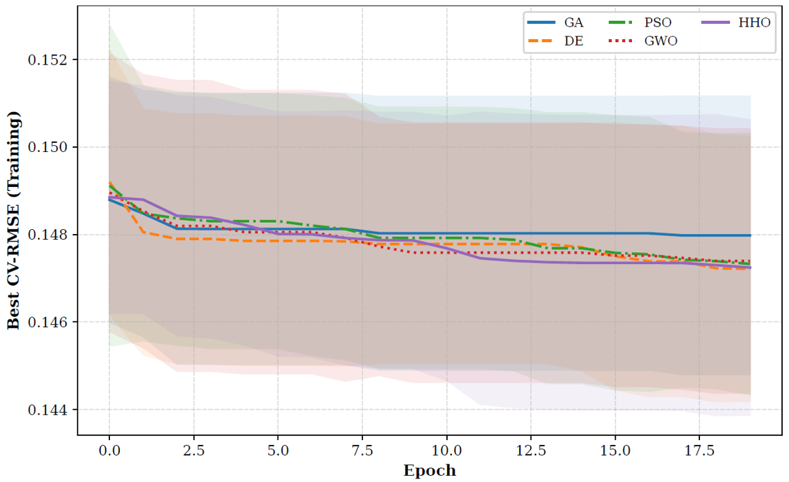
Figure 2 presents the convergence curves of the five metaheuristic algorithms, showing the best cross-validated RMSE achieved on the training set as a function of iteration number, averaged across five independent runs. All five algorithms show a general decreasing trend in the objective function value across iterations, confirming that each algorithm improves the MLP hyperparameter configuration over successive iterations.
Figure 2. Convergence curves of the five metaheuristic algorithms
GA converged fastest, reaching a near-stable plateau by approximately iteration 3–4. However, this rapid convergence came at a cost: GA achieved the smallest total reduction in objective value across the full search (0.00081), compared to 0.00198 for DE. This pattern suggests premature convergence, where the population loses diversity too early, and the search settles into a limited region of the hyperparameter space before adequately exploring alternatives. This behavior is consistent with the higher run-to-run variability observed for GA on the test set, discussed in Section 3.3.
In contrast, DE, PSO, and HHO continued to improve steadily well into the later iterations, with DE still showing measurable gains as late as iteration 18. Averaged across the five runs, DE achieved the lowest mean training RMSE (0.1472), followed closely by HHO (0.1472) and PSO (0.1473); GWO followed with 0.1474, while GA showed the highest mean training RMSE (0.1480). Table 5 separately reports the hyperparameter configuration of the single best-performing run per algorithm (selected by test R²), which does not necessarily correspond to the lowest training RMSE, since the two are optimized on different criteria, cross-validated training RMSE during search versus final test-set accuracy after refitting.
Table 5. Training CV-RMSE and hyperparameter configuration of the best solution per algorithm (mean ± std over 5 runs)
|
Algorithm |
CV-RMSE |
n1 |
n2 |
n3 |
Alpha |
lr |
|
GA |
0.1444 |
84 |
99 |
40 |
0.005370 |
0.009246 |
|
DE |
0.1526 |
53 |
9 |
30 |
0.000021 |
0.000861 |
|
PSO |
0.1469 |
28 |
44 |
34 |
0.001464 |
0.005137 |
|
GWO |
0.1527 |
128 |
41 |
64 |
0.000549 |
0.010000 |
|
HHO |
0.1462 |
110 |
105 |
17 |
0.026785 |
0.002594 |
3.3 Prediction performance on test set
Table 6 presents the mean and standard deviation of all seven-evaluation metrics across five independent runs for each algorithm on the independent test set. The results indicate that GWO achieved the highest overall prediction accuracy, with mean R² of 0.5836 ± 0.0031, RMSE of 0.8106 ± 0.0030 kWh/m², MAE of 0.5821 ± 0.0068 kWh/m², MAPE of 1.2558 ± 0.0145%, NSE of 0.5836 ± 0.0031, and Willmott’s d of 0.8540 ± 0.0044. These values indicate that the GWO-optimized MLP predicts cooling load with the best overall accuracy among the algorithms evaluated, although with modest absolute explanatory power (R² ≈ 0.58), a limitation discussed further in Section 3.7.
Table 6. Test set performance metrics for each algorithm (mean ± std over 5 runs)
|
Algorithm |
R2 |
RMSE |
MAE |
MAPE (%) |
Max Error |
NSE |
Willmott’s d |
|
GA |
0.5747 ± 0.0153 |
0.8192 ± 0.0145 |
0.5885 ± 0.0156 |
1.2685 ± 0.0319 |
2.9790 ± 0.1534 |
0.5747 ± 0.0153 |
0.8518 ± 0.0052 |
|
DE |
0.5768 ± 0.0024 |
0.8173 ± 0.0023 |
0.5797 ± 0.0047 |
1.2497 ± 0.0108 |
3.0128 ± 0.1561 |
0.5768 ± 0.0024 |
0.8552 ± 0.0028 |
|
PSO |
0.5772 ± 0.0035 |
0.8169 ± 0.0034 |
0.5899 ± 0.0093 |
1.2720 ± 0.0215 |
2.9262 ± 0.1760 |
0.5772 ± 0.0035 |
0.8512 ± 0.0047 |
|
GWO |
0.5836 ± 0.0031 |
0.8106 ± 0.0030 |
0.5821 ± 0.0068 |
1.2558 ± 0.0145 |
2.8706 ± 0.1277 |
0.5836 ± 0.0031 |
0.8540 ± 0.0044 |
|
HHO |
0.5580 ± 0.0113 |
0.8352 ± 0.0106 |
0.6255 ± 0.0218 |
1.3488 ± 0.0492 |
2.8156 ± 0.1266 |
0.5580 ± 0.0113 |
0.8452 ± 0.0067 |
GWO and PSO consistently ranked among the top performers across most metrics. Both algorithms are swarm-based, meaning each candidate solution updates its position using information from the best solutions found elsewhere in the population. This shared-information mechanism likely contributed to their stronger, more consistent performance than the evolutionary algorithms (GA, DE) tested in this study.
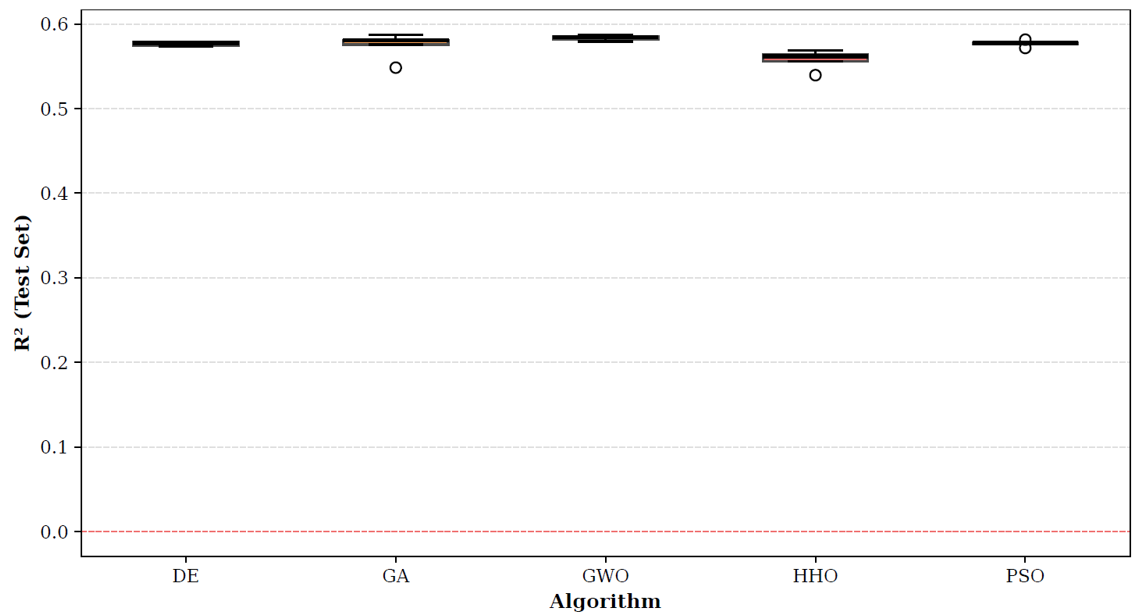
GA showed the highest run-to-run variability in test R² (std = 0.0153), more than four times that of DE (std = 0.0024). DE was the most stable and reproducible algorithm across independent runs. Interestingly, GA and DE are both evolutionary algorithms, yet they sit at opposite ends of the stability range. Algorithm category alone does not explain this difference. A more likely cause is GA’s crossover and mutation operators, which tend to produce less consistent exploration across different random initializations than DE’s difference-vector mutation strategy.
Figure 3 shows the boxplot distribution of R² across five runs for each algorithm. DE had the narrowest interquartile range, again confirming its stability. GA had the widest spread, suggesting its final solution quality depends more heavily on the search’s random initialization.
Figure 3. Boxplot distribution of coefficient of determination (R²) across five independent runs for each algorithm
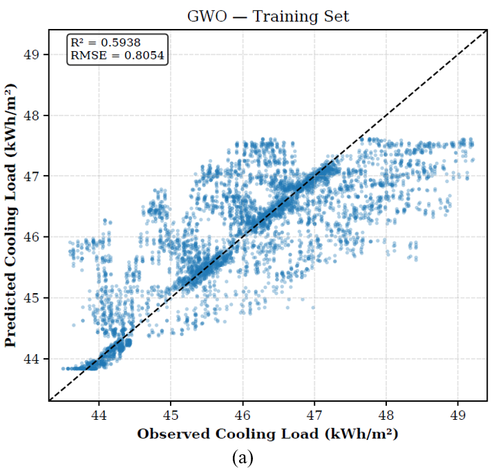
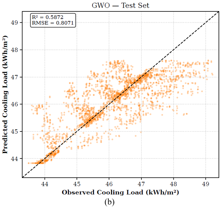
Figure 4 presents the scatter plots of predicted versus observed cooling load values for the best-performing algorithm (GWO) on the training and test sets. The predicted values closely follow the diagonal line of perfect agreement, with no systematic over-prediction or under-prediction evident across the range of observed values.
Figure 4. Predicted versus observed cooling load using the best-performing algorithm (GWO): (a) training set, (b) test set
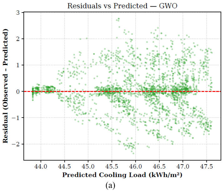
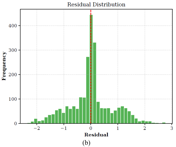
Figure 5 presents the residual analysis for the GWO model, showing residuals plotted against predicted values and the corresponding residual distribution. The residuals are approximately symmetric around zero with no strong systematic trend across the range of predicted values, indicating the absence of major systematic bias in the model predictions.
Figure 5. Residual analysis for the best-performing algorithm (GWO): (a) residuals versus predicted values, (b) residual distribution
3.4 Feature importance analysis
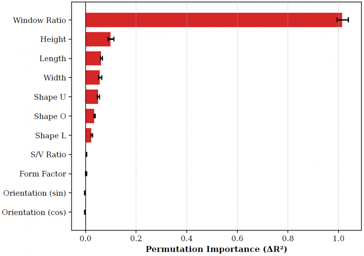
To identify which design variables strongly influence cooling load predictions, permutation feature importance was computed for the best-performing model (GWO) on the test set. Table 7 and Figure 6 present the ranked importance of each input feature, measured as the mean decrease in R² when the feature values are randomly permuted.
Table 7. Permutation feature importance (ΔR²) for the best-performing algorithm (GWO), ranked by mean importance across 10 permutation repeats
|
Feature |
Importance (Mean) |
Importance (Std) |
|
Window Ratio |
1.0166 |
0.0222 |
|
Height |
0.1010 |
0.0116 |
|
Length |
0.0632 |
0.0040 |
|
Width |
0.0584 |
0.0066 |
|
Shape U |
0.0515 |
0.0045 |
|
Shape O |
0.0364 |
0.0023 |
|
Shape L |
0.0252 |
0.0033 |
|
S/V Ratio |
0.0038 |
0.0010 |
|
Form Factor |
0.0025 |
0.0020 |
|
Orientation (sin) |
-0.0024 |
0.0008 |
|
Orientation (cos) |
-0.0029 |
0.0006 |
Figure 6. Permutation feature importance (ΔR²) for the best-performing algorithm (GWO)
The results show that WINDOWS_RATIO overwhelmingly dominates prediction accuracy, with permutation importance more than an order of magnitude higher than any other feature. Because R2 is not bounded below, permuting a dominant feature can drive model predictions below a naive mean-based baseline, producing a permuted R² lower than zero. For Window Ratio, the permuted R² is approximately -0.4330 (0.5836 minus 1.0166), confirming that a ΔR² exceeding the baseline R² is a mathematically expected outcome of the permutation procedure rather than a computational error. The dominance of window-to-wall ratio observed here is consistent with established building physics and prior simulation-based studies. WWR directly governs solar heat gain through glazing, which is the primary driver of cooling demand in tropical and hot-humid climates. Li et al. [18] demonstrated a near-linear increase in cooling-energy demand as WWR increased from 0% to 100% in a coupled microclimate-building energy simulation.
3.5 Statistical comparison
The Friedman test was applied to the RMSE values of all five algorithms across five independent runs to assess whether the observed performance differences are statistically significant. The test yielded a Friedman statistic of 13.44 and a p-value of 0.0093. Since the p-value is lower than the significance level of 0.05, the null hypothesis that all algorithms perform equally is rejected. This result indicates that the observed differences in prediction accuracy among the five algorithms are statistically significant, and that the ranking of algorithms reported in Table 6 reflects genuine performance differences rather than random variation. Post-hoc Wilcoxon signed-rank tests comparing GWO against each of the remaining algorithms showed a consistent directional advantage for GWO, which outperformed DE, HHO, and PSO in all five paired runs (p = 0.0625 for each comparison). However, these pairwise comparisons did not reach the conventional significance threshold individually, a limitation attributable to the maximum achievable precision of the exact Wilcoxon test at n = 5 rather than to a weak underlying effect.
3.6 Implications for early-stage building design
The results show that metaheuristic-optimized MLP models can reliably predict cooling load for open courtyard configurations at the early design stage. These configurations comprise L-shape and U-shape. Predictive reliability for the fully enclosed O-shape configuration remains constrained. The dataset limitations discussed below explain this constraint. The model requires only basic morphological and envelope parameters. This information is typically available before detailed design documentation is complete. The best-performing model was optimized using GWO. This model achieved an R² of 0.5836 on the independent test set. It achieved an RMSE of 0.8106 kWh/m² on the same set. The selected input features explain roughly 58% of the variance in cooling load.
These findings carry practical value for architectural design workflows. A trained MLP model can be embedded in early-stage design decision support tools. Designers can use these tools to quickly screen open courtyard configurations. Designers can identify configurations with lower cooling demand before committing them to a specific design direction. This approach is faster than running a full energy simulation for every design variant. It does not require specialist energy modeling expertise from the designer.
This study examined three courtyard shapes. These shapes are L-shape, O-shape, and U-shape. The shapes differ in enclosure degree and self-shading capacity. Both factors influence solar heat gain within the courtyard space. Both factors also influence natural ventilation within the courtyard space. O-shape is the fully enclosed configuration. O-shape recorded the highest mean cooling load at 46.22 kWh/m². U-shape is the more open configuration. U-shape recorded the lowest mean cooling load at 45.61 kWh/m². This result runs counter to a common assumption. The assumption holds that greater enclosure reduces cooling demand through increased self-shading. A plausible explanation involves ventilation. Full enclosure also restricts natural ventilation within the courtyard. This restriction traps heat inside the courtyard. The trapped heat would otherwise dissipate through cross-ventilation in more open configurations such as U-shape. The dataset is also imbalanced across shape. O-shape comprises 64% of all samples. This imbalance may itself contribute to the wider spread of cooling load values observed for O-shape. The standard deviation for O-shape reaches 1.30. The standard deviation for both L-shape and U-shape reaches only 1.11. This finding suggests an interaction between courtyard enclosure and ventilation performance. Solar exposure alone does not capture this interaction. Section 3.7 makes the case for incorporating airflow and ventilation-related variables in future extensions of this dataset. This finding reinforces that case.
Per-shape evaluation of the best-performing model on the test set clarifies this imbalance further. L-shape is predicted with high accuracy. L-shape reaches an R² of 0.9913 and an RMSE of 0.1042 kWh/m². U-shape is also predicted with high accuracy. U-shape reaches an R² of 0.9883 and an RMSE of 0.1213 kWh/m². O-shape is predicted with substantially lower accuracy. O-shape reaches an R² of only 0.3892 and an RMSE of 1.0048 kWh/m². This disparity traces to the underlying dataset rather than to model capacity or training imbalance. The O-shape subset contains 1,514 unique combinations of the seven geometric input features. Among these, 1,481 combinations correspond to multiple samples with differing cooling load values. The pooled within-combination variance accounts for approximately 79% of total O-shape target variance. This finding is consistent with the correlation pattern between window-to-wall ratio and cooling load. This correlation reaches 0.97 for both L-shape and U-shape. This correlation reaches only 0.55 for O-shape. These results indicate a missing geometric degree of freedom specific to the fully enclosed configuration. The internal courtyard aperture dimension most plausibly represents this missing factor. The present input features do not capture this factor. This gap imposes a data-driven ceiling on achievable predictive accuracy for O-shape. This ceiling is independent of model architecture or hyperparameter tuning. Predictive claims regarding this MLP-based approach should therefore be scoped to open courtyard configurations. These configurations comprise L-shape and U-shape. This scope should hold until an aperture-related predictor can be incorporated for the fully enclosed case.
The absolute range of cooling load in this dataset is also narrow. This range spans 43.50 to 49.21 kWh/m². The standard deviation reaches 1.26. This narrow range constrains the practical magnitude of difference an R² of 0.58 can represent. In absolute terms, however, the best-performing model achieves an RMSE of 0.81 kWh/m². This RMSE corresponds to approximately 14% of the observed range. This magnitude remains practically informative for comparative design screening. R² itself appears modest despite this. Differences in R² at the third decimal place between algorithms should therefore be interpreted carefully. GWO reaches 0.5836. PSO reaches 0.5772. These differences indicate relative algorithm consistency. These differences do not indicate meaningfully different real-world prediction accuracy. Section 3.5 reports the Friedman and Wilcoxon tests. These tests address this distinction directly. These tests examine rank consistency across runs. These tests do not examine the practical magnitude of difference between algorithms.
The best hyperparameter configurations identified for several algorithms also reached the boundary of the defined search space. GWO’s optimal number of neurons in the first hidden layer reached 128. GWO’s optimal learning rate reached 0.01. Both values correspond to the upper bounds reported in Table 2. This raises the possibility that better-performing configurations exist outside the explored range. The present search already incurred substantial computational cost. Section 2.6 describes this cost. The search space was not extended further in this study. This saturation is instead noted here as a limitation. Future work should verify whether relaxing these bounds yields additional accuracy gains.
3.7 Beyond window-to-wall ratio: Toward a more comprehensive cooling load model
In general, cooling loads in tropical regions are strongly influenced by design and non-design factors. Non-design factors such as occupancy level, occupancy behavior, and building function can only be determined effectively during operation. However, design factors such as window design, building facades, and material types can influence architects’ design decisions [19]. This decision is especially insightful when supported by early cooling-load estimates before construction starts. It also aligns with this study’s finding, as shown in Figure 6, that the most important feature influencing courtyard building cooling-load prediction is the WWR. Because design factors are so important, future studies should explore combinations of design factors, including WWR ratios, glazing types and specifications, building envelope properties, color, and shading, to generate lower cooling-load predictions.
In addition, extending the prediction with hourly historical climate and outdoor temperature data measured specifically in the Shah Alam microclimate will provide more accurate estimates and support solid design decisions. Extending the dataset in this direction would allow future metaheuristic-optimized models to unravel the relative contributions of morphological design decisions (the focus of the present study) from envelope material to climate-driven factors. This will provide architects and building designers in regions with comparable tropical contexts with a more complete, physically grounded basis for early-stage cooling load estimation. Furthermore, direct comparison between the courtyard-shape-driven design strategies and retrofits involving building’s envelope-level interventions (e.g., low-SHGC glazing, external shading) is not possible within the scope of the present dataset. Thus, metaheuristic-optimized MLP models can help support informed design decisions in the future.
3.8 Economic implications of metaheuristic-optimized early-stage prediction
Beyond its technical contribution, the practical value of a metaheuristic-optimized MLP model for cooling load prediction lies in its potential to reduce the cost and time associated with early-stage building energy assessment. Detailed dynamic energy simulation using tools such as IESVE typically requires substantial input preparation, computational runtime, and specialist expertise, incurring direct consultancy costs that are often difficult to justify for architects and developers during the conceptual design phase, when multiple design alternatives are still being compared under tight budget and schedule constraints. The trained MLP model developed in this study produces a cooling load estimate in a fraction of a second once optimized, compared with the substantially longer setup and computation time typically required for a single detailed simulation run in dynamic energy modeling software [20]. This order-of-magnitude reduction in evaluation time and required expertise lets developers and design teams screen far more courtyard configurations within the same design timeline and consultancy budget, potentially reducing the direct cost of the design exploration phase and enabling earlier identification of lower-cooling-load design options before capital-intensive detailed design work begins. Because cooling load is directly proportional to ongoing HVAC operating expenditure over a building’s service life, design decisions informed at this early, low-cost screening stage carry disproportionate downstream economic value relative to their marginal assessment cost, as design changes become progressively more expensive to implement as a project moves toward construction documentation.
This study compared five metaheuristic optimizers for tuning an MLP model used to predict cooling-load intensity for tropical courtyard buildings. The comparison was designed to examine different search mechanisms under a common MLP architecture and broadly comparable optimization settings. Using 8,535 parametric simulation samples and five stochastic runs per optimizer, GWO produced the highest mean test-set R² of 0.5836, and the lowest mean RMSE of 0.8106 kWh/m². Meanwhile, DE showed the smallest run-to-run variation in R² with 0.0024 std. The Friedman test indicated overall differences in algorithm rankings (p = 0.0093), but the five-run design limited the strength of pairwise inference, and the small absolute differences among the leading optimizers should not be overstated. Permutation importance identified WWR as the dominant predictor among the recorded features. More importantly, the per-shape analysis showed that predictive performance was very high for the L- and U-shaped configurations but substantially weaker for the fully enclosed O-shape, in which repeated combinations of predictors yielded different cooling-load values. This pattern indicates missing information in the current feature set and supports the inclusion of additional courtyard geometry, glazing, shading, airflow, and climate variables in future datasets. The present model is therefore best viewed as an early-stage screening surrogate for the open-courtyard configurations represented in the data, rather than as a replacement for detailed simulation or a universally transferable predictor. Future validation should also use grouped or repeated outer splits that keep identical design combinations together, select hyperparameters without reference to the test set, and use more stochastic runs before drawing stronger conclusions about differences among optimizers.
This research was funded by Institute of Research and Community Service (LPPM) Universitas Negeri Semarang under contract No. 735.8.4/UN37/PPK.11/2026.
[1] Cao, X., Dai, X., Liu, J. (2016). Building energy-consumption status worldwide and the state-of-the-art technologies for zero-energy buildings during the past decade. Energy and Buildings, 128: 198-213. https://doi.org/10.1016/j.enbuild.2016.06.089
[2] Kajjoba, D., Wesonga, R., Lwanyaga, J.D., Kasedde, H., Olupot, P.W., Kirabira, J.B. (2025). Assessment of thermal comfort and its potential for energy efficiency in low-income tropical buildings: A review. Sustainable Energy Research, 12: 25. https://doi.org/10.1186/s40807-025-00169-9
[3] Al-Shargabi, A.A., Almhafdy, A., Ibrahim, D.M., Alghieth, M., Chiclana, F. (2021). Tuning deep neural networks for predicting energy consumption in arid climate based on buildings characteristics. Sustainability, 13(22): 12442. https://doi.org/10.3390/su132212442
[4] Aloshan, M.A., Aldali, K.M. (2025). Courtyard design for energy efficiency and thermal comfort: Machine learning insights across hot and warm climates. Scientific Reports, 15(1): 43660. https://doi.org/10.1038/s41598-025-32297-z
[5] Yan, Z., Zhu, X., Wang, X., et al. (2023). A multi-energy load prediction of a building using the multi-layer perceptron neural network method with different optimization algorithms. Energy Exploration & Exploitation, 41(1): 273-305. https://doi.org/10.1177/01445987221112250
[6] Del Ama Gonzalo, F., Moreno Santamaría, B., Montero Burgos, M.J. (2023). Assessment of building energy simulation tools to predict heating and cooling energy consumption at early design stages. Sustainability, 15(3): 1920. https://doi.org/10.3390/su15031920
[7] Li, L., Qi, Z., Ma, Q., Gao, W., Wei, X. (2024). Evolving multi-objective optimization framework for early-stage building design: Improving energy efficiency, daylighting, view quality, and thermal comfort. Building Simulation, 17(11): 2097-2123. https://doi.org/10.1007/s12273-024-1178-6
[8] Villano, F., Mauro, G.M., Pedace, A. (2024). A review on machine/deep learning techniques applied to building energy simulation, optimization and management. Thermo, 4(1): 100-139. https://doi.org/10.3390/thermo4010008
[9] Xu, Y., Li, F., Asgari, A. (2022). Prediction and optimization of heating and cooling loads in a residential building based on multi-layer perceptron neural network and different optimization algorithms. Energy, 240: 122692. https://doi.org/10.1016/j.energy.2021.122692
[10] Karbasforoushha, M.A., Khajehzadeh, M., Jearsiripongkul, T., Keawsawasvong, S., Eslami, M. (2024). A comprehensive review of building energy optimization using metaheuristic algorithms. Journal of Building Engineering, 98: 111377. https://doi.org/10.1016/j.jobe.2024.111377
[11] Yuan, X., Karbasforoushha, M.A., Syah, R.B., Khajehzadeh, M., Keawsawasvong, S., Nehdi, M.L. (2022). An effective metaheuristic approach for building energy optimization problems. Buildings, 13(1): 80. https://doi.org/10.3390/buildings13010080
[12] Zheng, S., Lyu, Z., Foong, L.K. (2022). Early prediction of cooling load in energy-efficient buildings through novel optimizer of shuffled complex evolution. Engineering with Computers, 38(Suppl 1): 105-119. https://doi.org/10.1007/s00366-020-01140-6
[13] Afzal, S., Shokri, A., Ziapour, B.M., Shakibi, H., Sobhani, B. (2024). Building energy consumption prediction and optimization using different neural network-assisted models; comparison of different networks and optimization algorithms. Engineering Applications of Artificial Intelligence, 127: 107356. https://doi.org/10.1016/j.engappai.2023.107356
[14] Mu, W., Cardelli, R., Ferrari, S. (2026). Data preprocessing techniques for machine learning towards improving building energy performance: A systematic review. Energies, 19(6): 1561. https://doi.org/10.3390/en19061561
[15] Almhafdy, A., Al-Mutairi, A., Al-Shargabi, A., Al-Shargabi, A. (2025). Dataset on energy consumption in buildings within tropical climate based on design aspects of courtyards. Data in Brief, 61: 111834. https://doi.org/10.1016/j.dib.2025.111834
[16] Al Bataineh, A., Kaur, D., Jalali, S.M.J. (2022). Multi-layer perceptron training optimization using nature inspired computing. IEEE Access, 10: 36963-36977. https://doi.org/10.1109/ACCESS.2022.3164669
[17] Brest, J., Sepesy Maučec, M. (2025). Comparative study of modern differential evolution algorithms: Perspectives on mechanisms and performance. Mathematics, 13(10): 1556. https://doi.org/10.3390/math13101556
[18] Li, J., Zheng, B., Bedra, K.B., Li, Z., Chen, X. (2021). Evaluating the effect of window-to-wall ratios on cooling-energy demand on a typical summer day. International Journal of Environmental Research and Public Health, 18(16): 8411. https://doi.org/10.3390/ijerph18168411
[19] Tan, X.Y., Mahyuddin, N., Zaid, S.M. (2023). Efficacy of energy conservation measures and building energy intensity of a multi-building complex in Malaysia. E3S Web of Conferences, 396: 03004. https://doi.org/10.1051/e3sconf/202339603004
[20] Shirzadi, N., Lau, D., Stylianou, M. (2025). Surrogate modeling for building design: Energy and cost prediction compared to simulation-based methods. Buildings, 15(13): 2361. https://doi.org/10.3390/buildings15132361