Seismicity Clustering and Coulomb Stress Analysis of the Palu-Koro Fault

2.1 Geological setting

The island of Sulawesi lies within a complex tectonic zone influenced by the interaction of several major plates and microblocks, including the Indo-Australian Plate, the Philippine-Pacific Plate, and the Sunda Block. This tectonic complexity has led to the formation of a network of active faults, subduction systems, microblock rotation, and significant crustal deformation. In West and Central Sulawesi, the Palu-Koro Fault is the main structure accommodating left-lateral deformation and serves as one of the primary boundaries between tectonic blocks [20].

The Palu-Koro Fault extends from a north-west to south-east direction to an almost north-south orientation, stretching from the offshore area of Palu Bay through Palu to the southern part of Central Sulawesi. The geometry of this fault is complex due to bends in its segments, branching structures, and its possible interconnection with surrounding fault systems. Previous studies on the 2018 Palu earthquake indicate that the fault zone can rupture across multiple segments, suggesting that segmentation is a key factor in determining earthquake hazard at this location [21].

Geological formations play a crucial role in earthquake studies in the Palu-Koro Fault region, which includes Quaternary alluvial deposits (Qa) [2, 22], metamorphic rock complexes (Tm) [23, 24], and Tertiary sedimentary rocks (Tmtv/Tmpb) [24, 25] (see Figure 1). The Quaternary alluvial deposits (Qa) in the Palu Basin consist of loose materials such as sand, gravel, and clay that are poorly consolidated; as a result, they can amplify seismic waves and increase liquefaction potential. The metamorphic rock complex (Tm) and Tertiary sedimentary rocks (Tmtv/Tmpb/Tmb) are the primary constituent rocks that have undergone deformation due to tectonic activity along the Palu-Koro Fault, thereby acting as zones for the accumulation and release of seismic energy [26, 27]. The combination of active faults and the characteristics of these rock formations makes this region highly vulnerable to earthquake hazards. These characteristics are important not only for earthquake hazard assessment, but also for the management of degraded land, spatial planning, and infrastructure development in regions with tectonic activity [28].

tu_pian_12.png

2.2 Earthquake data

In this study, we used data from the local earthquake catalog of the BMKG network (http://geof.bmkg.go.id/webdc3/) covering the period from 1 January 2011 to 31 December 2015 in the Palu-Koro Fault and surrounding areas. The earthquake data comprised 398 events with magnitudes ≥ Mw 3, recorded by 21 BMKG stations (Figure 2). The selected timeframe covers the periods before, during, and after the Mw 6.3 earthquake on 18 August 2012, enabling this analysis to encompass both background seismicity and the post-mainshock aftershock sequence. The earthquake parameters included are time of occurrence, epicenter location, depth, magnitude, and arrival times of P- and S-waves, which were manually selected using NonLinLoc as the basis for analyzing the hypocenter distribution [10]. NonLinLoc was chosen because it employs a probabilistic, non-linear, and global search approach, enabling estimation of the hypocenter location and its spatial uncertainty, particularly in regions with complex velocity structures. The NLLoc program generates a misfit function that identifies the 'ideal' hypocenter by determining the probability density function (PDF). Utilize a PDF to ascertain the coordinates of the x, y, and z hypocentres employing one of the following methods: grid search systematic, stochastic Metropolis-Gibbs method, or oct-tree significance sampling techniques [11].

tu_pian_13.png

Figure 2. The distribution of earthquake events around the Palu-Koro Fault, both before and after the Mw 6.3 earthquake on 18 August 2012

Meanwhile, the fault plane parameters (strike = 339°, dip = 82°, and rake angle = -5°) were obtained from the Global CMT catalog (https://www.globalcmt.org/) (Figure 2) to determine the length and width of the fault using calculations carried out for strike-slip faults [30]. This estimation process utilized the Coulomb 3.4 program [31, 32]. In this estimation, the input parameters used were Poisson’s ratio ($v$) = 0.25, Young’s modulus (E) = 800,000 bar, and effective friction coefficient ($\mu^{\prime}$) = 0.4.

2.3 Hierarchical Density-Based Spatial Clustering of Applications with Noise clustering

The HDBSCAN clustering method is an extension of DBSCAN, utilizing a density-based, hierarchical algorithm. One of the advantages of this algorithm is its ability to handle clusters of various shapes, high dimensions, and an uncertain number of clusters; there is no need to specify an ideal number of clusters in advance, making this clustering method suitable for spatial data [18, 19, 33]. The main differences between HDBSCAN and DBSCAN lie in the distance function and the hierarchical structure, which is constructed based on the density between data points.

tu_pian_14.jpg

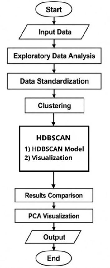
Figure 3. Flowchart model for earthquake data analysis using Hierarchical Density-Based Spatial Clustering of Applications with Noise (HDBSCAN) clustering

The flowchart (Figure 3) illustrates the workflow for earthquake clustering analysis using an unsupervised machine learning method, namely HDBSCAN clustering. The dataset contains three main variables: longitude, latitude, and earthquake depth. Initial exploration using the header (data) and summary (data) indicates that longitude values range from 117.3 to 122.1, latitude values range from -4.369 to 4.396, and earthquake depth values range from 1.089 km to 285.836 km, with an average depth of approximately 55.989 km.

Prior to clustering, longitude, latitude, and hypocentral depth were standardized using z-score normalization to remove differences in numerical scale. HDBSCAN was then applied to the standardized three-dimensional feature space using the default Euclidean distance metric implemented in the R dbscan package with minPts = 10. Following the original HDBSCAN algorithm, mutual reachability distances were first computed to account for local density differences, after which a minimum spanning tree (MST) was constructed. The hierarchical cluster tree was subsequently pruned based on cluster stability, and the most stable clusters were automatically extracted without requiring a predefined number of clusters.

We applied the HDBSCAN method directly to the standardized data with a minPts value of 10. HDBSCAN automatically determines the number of clusters and identifies observations that are noise or outliers. The analysis yielded four main clusters and one noise group (cluster 0). The resulting distribution comprises 195 observations classified as noise/outliers, whilst the remaining observations form clusters containing 15, 21, 16, and 151 earthquake events, respectively. The large number of noise points indicates that the earthquake distribution exhibits a heterogeneous, non-linear spatial pattern, which is common in seismic data from active fault systems with varying tectonic activity.

Following the clustering stage, the HDBSCAN method distinguishes dense seismic regions from rare events or anomalies. This feature makes HDBSCAN more flexible in identifying irregular seismic patterns and unusual earthquakes. Spatial visualizations are then generated using longitude and latitude coordinates to illustrate the distribution of the resulting earthquake clusters. Next, to further evaluate the cluster structure, we performed a principal component analysis (PCA) on the standardized dataset. PCA reduces multidimensional data using the first and second-highest Eigenvalues, allowing clustering patterns to be visualized in a lower-dimensional space. The resulting PCA plot from the HDBSCAN clustering was used to visualize cluster separation and data distribution patterns better. Consequently, the clustering results, including the cluster labels, were exported for further interpretation and seismic analysis.

2.4 Coulomb stress

In determining the source-fault inputs, we used several earthquake parameters, namely the epicentre coordinates, depth, magnitude, and strike, dip, and rake. Fault dimensions such as length (L), width (W), area (A), and displacement (D) were analysed using the empirical relationship [30] intended for thrust faults. Coulomb stress calculations were performed over a depth range of 0 to 30 km, at 5 km intervals. This depth range was selected based on the hypocenter of the main earthquake, located at approximately 13 km depth.

Assuming a simple Coulomb friction model for earthquakes, the potential slip will increase or decrease with ΔCFS [34], which is defined as Eq. (1):

$\triangle C F S=\triangle \tau+\mu^{\prime} \triangle \sigma_\sigma$       (1)

where ∆CFS is the Coulomb failure stress, ∆τ denotes the shear stress, $\Delta \sigma_n$ indicates the sum of the normal stress and fluid pore pressure (P), and $\mu^{\prime}$ is the effective friction coefficient. The normal stress is positive when the fault is unlocked and negative when it is locked, whilst the shear stress is positive for slip in the slip direction.

The value of P modifies the effective normal stress along the fault plane. When rock stress changes rapidly, P subsequently changes in a flow-like manner. The value of P can be related to Skempton’s coefficient B, which varies between 0 and 1. The effective friction coefficient in coseismic stress studies ranges from 0.01 to 0.75, with an average of $\mu^{\prime}$ = 0.4. ∆CFS is resolved on the first fault plane and in the direction of slip on the second fault plane or the receiver fault.

Where the effective stiffness is expressed as $\mu^{\prime}$ = µ(1 - β); furthermore, if ∆CFS > 0, the slip potential will increase, and if ∆CFS < 0, the slip potential will decrease. The calculation of ∆CFS caused by an earthquake depends on the geometry and distribution of slip, the assumed magnitude, the regional stress orientation, and the value of the assumed stiffness. The ratio of regional stress amplitude to earthquake stress drop has a significant impact only near the fault. In some cases, the uncertainty in ∆CFS is always dominated by that in the slip distribution. In principle, if ∆CFS > 0 (positive), it means that the first fault can cause the second fault to experience an increase in stress, making the likelihood of failure on the second fault greater. Conversely, if ∆CFS < 0 (negative), the first fault relaxes the second fault, thereby reducing the likelihood of failure; this region is often referred to as a stress shadow zone.

To strengthen the analytical framework, this study integrates deterministic geomechanical modelling and data-driven clustering techniques. Coulomb stresses were calculated using the Coulomb 3.4 software [31, 32], which is based on the theory of elastic dislocations in a homogeneous half-space. This model estimates the Coulomb Failure Stress (ΔCFS) as a function of the shear stress change (Δτ), the normal stress change (Δσ_n), and the effect of pore-fluid pressure on an optimally oriented host fault. In this study, the Coulomb 3.4 software was applied to simulate the co-seismic stress disturbance associated with the Mw 6.3 Palu-Koro earthquake, using fault geometries derived from Global CMT solutions and empirical scaling relationships. Stress variations were evaluated at depth intervals of 0-30 km to capture vertical heterogeneity relevant to the hypocentre distribution. Positive ΔCFS values indicate stress loading and an increased potential for failure, whilst negative values represent stress-shadow zones that inhibit crack initiation. To identify spatial patterns, earthquake hypocentres were analysed using HDBSCAN [17, 18, 33] in R, with a minimum cluster size of 10. HDBSCAN identifies clusters of varying density without requiring a predefined number of clusters, making it suitable for irregular seismic distributions. This method distinguishes the dense core of earthquakes from background seismicity and noise. The combined use of Coulomb stress modelling and HDBSCAN clustering provides a highly complementary framework that links physical stress transfer with the structure of statistical seismicity.

The spatial correlation between the earthquake catalog and the ΔCFS grid was determined by superimposing the hypocenter coordinates onto the calculated Coulomb 3.4. For each earthquake, the relevant ΔCFS value was obtained from the grid node closest to the hypocenter, without using spatial interpolation. This methodology ensured that every seismic event was explicitly linked to a corresponding ΔCFS value derived from the calculated stress field for subsequent spatial and statistical analyses.

4.1 Hierarchical Density-Based Spatial Clustering of Applications with Noise analysis

HDBSCAN helps better understand areas with high earthquake density. The results show that the area around the epicentre of the 2012 earthquake is the most prominent region in the seismicity distribution. This indicates that the area is significant both as the location of a major earthquake and for consistently exhibiting high seismic activity throughout the analysis period. One of the key strengths of HDBSCAN is its ability to distinguish between large clusters and low-density seismic activity. This distinction is crucial in earthquake analysis. Each earthquake has a different structural significance. Certain events may appear as background activity, whilst others may form part of a consistent active pattern. HDBSCAN separates dense clusters from background noise.

Based on the HDBSCAN map (Figure 4), the concentration of high values around the Palu-Koro Fault zone indicates that this major fault structure controls seismic activity. This is consistent with the fact that the Palu-Koro Fault is one of the most active left-lateral strike-slip faults in Indonesia. Recent integrated studies of gravity, GNSS, and seismic data also show that the Palu-Koro is a highly active left-lateral strike-slip fault and plays a key role in the tectonic framework of Central Sulawesi [27]. Consequently, the earthquake density analysed by HDBSCAN can be linked to crustal deformation processes occurring throughout this fault system.

Furthermore, seismic activity is not concentrated in a single location, as demonstrated by the HDBSCAN clustering results (Figure 5). These areas are scattered along the fault, with some extending southwards. This pattern may indicate a relationship between the main segment of the Palu-Koro Fault and local structures in Central Sulawesi. In the context of earthquake hazard, this information is important, as areas with high seismicity can be prioritised for more detailed seismic monitoring.

4.2 Coulomb stress analysis

Coulomb stress analysis provides a mechanical explanation for the seismicity patterns in the study area. In this study, many hypocentres are located near zones of positive Coulomb stress. This suggests that the stress changes caused by the mainshock, as interpreted, contribute to the distribution of earthquakes following the mainshock. Areas with a higher tendency for shear failure are known as positive Coulomb stress zones. This mechanical interpretation is further supported by clusters of seismic activity surrounding these areas. In other words, these clusters may be caused by physical stress changes in the Earth’s crust as well as the proximity of seismic events to one another. This relationship is crucial for understanding the patterns of seismic activity that persist following a major earthquake.

However, not all clusters need to coincide perfectly with the positive stress lobes. Some earthquake epicentres may appear in the transition zone or near the negative stress zone on the map, or even near negative stress zones on the map, though not significantly so. This is likely due to a lack of rupture in those areas, causing them to experience a stress shadow. Given the uncertainty of the Coulomb stress model, this is indeed to be expected. Parameters such as fault plane orientation, the effective friction coefficient, source depth, and assumptions about the medium's elasticity significantly influence earthquake stress values. It has been demonstrated that the distribution of receiving fault planes, as well as spatiotemporal heterogeneity, can affect the results of Coulomb stress analysis [38].

For further analysis, we have divided the Coulomb stress field into several sections to present cross-sections illustrating the vertical stress distribution. As shown in Figure 7, we have used three cross-sections: A-B, C-D, and E-F. Cross-section A-B, which is parallel to the fault plane, and cross-section C-D, which is perpendicular to the fault plane, respectively show a dominant increase in stress (red areas) at depths of 0-10 km and 20-30 km, with a decrease in stress (blue areas) separating these two regions at a depth of 10-20 km (Figures 7(a) and (b)). There is also an increase in stress from depths of 0-30 km, as shown by cross-section E-F (northwest to southeast), which is perpendicular to the fault plane (Figure 7(c)). Cross-sections A-B and C-D show that the earthquakes (represented by points) are largely distributed within the areas of increased stress. However, because this earthquake was a strike-slip event, the distribution of earthquakes (presented by points) is generally spread across both the red and blue lobes (E-F).

Therefore, the interpretation of Coulomb stress in this study must be based on probabilistic and mechanistic approaches. These stress maps are not intended to pinpoint the exact location of the next earthquake, but rather to identify areas that are more likely to experience geological activity. In the context of Palu-Koro, the positive lobe area situated close to the main cluster is best described as an area experiencing a strong post-earthquake stress response.

4.3 Integration of Hierarchical Density-Based Spatial Clustering of Applications with Noise and Coulomb stress

This research does not limit itself to spatial mapping or mechanical interpretation in isolation; rather, it combines two methods with distinct epistemological foundations. Coulomb stress reflects the physical response of the Earth’s crust to the redistribution of stress caused by earthquakes, whilst HDBSCAN is a data-driven approach that extracts density structures without considering the shape of the distribution. The combination of the two provides a more robust interpretative framework for understanding post-earthquake mechanisms in the Palu-Koro fault system.

The HDBSCAN clustering results indicate that the distribution of hypocentres is inconsistent and tends to form seismic cores localized around the main Palu-Koro segment (Figure 5).

The quantitative distribution of earthquake data points, in both number and percentage, across the positive and negative DCFS is shown in Table 3. Note that because cluster 0 shows no clear spatial relationship with the Coulomb stress pattern (Figure 5), the cluster is classified as noise. Consequently, the cluster is not associated with the DCFS.

Table 3 demonstrates that hypocentres in Cluster 1 correlate with DCFS > 0, while Cluster 3 gives DCFS < 0. Cluster 2 is divided into two sections, one with a positive ACF and the other with a negative DCFS, in relatively equal numbers. Additionally, Cluster 4 has 44.33% correlated with DCFS positive and 30.05% related to DCFS negative.

Table 3. Quantitative distribution and percentage of earthquakes in each cluster

On the other hand, the Coulomb stress results indicate that the areas with these clusters are largely situated within zones of Coulomb Failure Stress (DCFS > 0). This spatial correlation suggests that structural heterogeneity and the transfer of static stress from the mainshock influenced the seismic activity following the Mw 6.3 earthquake [8]. Specifically, cluster 1 represents the dominant seismic concentration around the main fault and shows the strongest spatial correlation with the positive Coulomb stress region.

Each cluster exhibits a different distribution of earthquake occurrences with respect to changes in Coulomb stress (ΔCFS), as shown in Table 3. Overall, 110 earthquakes (54.19%) occurred in regions with higher Coulomb stress, while 93 earthquakes (45.81%) occurred in regions with lower Coulomb stress. This indicates that most earthquakes occur in areas with higher Coulomb stress, suggesting that fault planes are more likely to fail, particularly as Coulomb stress increases [34, 39].

With 151 earthquake events, or about 74.4% of the total, data cluster 4 was the most dominant. A total of 90 events (59.6%) in this cluster occurred in the ΔCFS > 0 region, while 61 events (40.4%) occurred in the ΔCFS < 0 region. The predominance of ΔCFS > 0 within the largest cluster suggests that seismic activity tends to concentrate in areas under increased stress. Previous studies have shown that static stress transfer can control the distribution of aftershocks and shift the location of subsequent earthquakes toward areas with increased Coulomb stress [39].

Nevertheless, the presence of 61 events in cluster 4 and all 16 events in cluster 3 occurring in regions with ΔCFS < 0 indicates that changes in Coulomb stress are not the sole factor controlling seismic activity. Changes in pore-fluid pressure, heterogeneity in the regional stress field, and the complexity of poorly defined fault geometries can still cause earthquakes to occur in areas with ΔCFS < 0. Furthermore, research conducted on the 2011 Tohoku Earthquake shows that increased seismic activity can also occur in areas conventionally considered to be under shadow stress, particularly at locations where fault systems have various orientations [32].

Although there were only five earthquakes, Cluster 1 was entirely located in the region where ΔCFS > 0, whereas Cluster 2 showed an almost balanced distribution between ΔCFS > 0 and negative values. The local stress conditions of each cluster differ, as indicated by their distinct characteristics. Therefore, the clustering results using HDBSCAN reveal various physical conditions that influence cluster formation and the spatial concentration of earthquakes.

Overall, the results in Table 3 show that clusters with the highest number of events are more likely to be associated with ΔCFS > 0, supporting the hypothesis that stress redistribution contributes to the development of seismic activity around the Palu-Koro Fault. In this case, cluster 0 was excluded because it was correlated with noise. However, the proportion of events in the ΔCFS < 0 region remains substantial, indicating that the interpretation of Coulomb stress must be integrated with other geological components. Therefore, a more comprehensive understanding of the spatial patterns of seismicity can be obtained by integrating HDBSCAN and Coulomb stress analysis rather than using the two methods separately.

This study broadens our understanding of the Palu-Koro Fault system, an active fault with complex segmentation. Seismic activity is not only concentrated around the epicenter, but also spreads in various directions along fault lines and structures surrounding the epicenter. This pattern suggests that the stability of several areas surrounding the source of the Mw 6.3 earthquake in 2012 may be compromised. These segments are of great importance for studies on earthquake hazard potential. Segments showing dense seismic clusters together with positive Coulomb stress conditions represent areas where stress loading and earthquake activity occur simultaneously, making them important targets for seismic hazard evaluation, as they are most likely to experience increased seismic activity following a major earthquake. Conversely, segments showing sparser clusters but still following fault structures should be regarded as transition zones or areas of moderate seismic activity.

The integration of probabilistic hypocentre relocation, density-based clustering (HDBSCAN), and Coulomb stress modeling within a single interpretation pipeline is the key strength of this method. This method enables cross-validation between statistical structures (cluster stability) and physical controls (stress transfer). The results not only indicate areas of concentrated earthquake activity but also provide further insight into why such spatial concentrations form.

One of the key benefits of this integration is the ability to identify fault segments that simultaneously exhibit high seismicity density and stress loading. In this study, Clusters 1, 2, and 4 represent conditions in which dense seismicity coincides with positive ΔCFS values. Conversely, clusters located outside the strongest stress-loading regions highlight the influence of additional geological factors beyond static stress transfer.