Nooraldeen Saleh Khidhir* | Yaser Shuker Mahmood | Ammar Younis Ibrahim | Abdulrahman Habbo Mohammed | Anwar Mohammed Mostafa | Mohamed Taktak | Mohamed Haddar
© 2026 The authors. This article is published by IIETA and is licensed under the CC BY 4.0 license (http://creativecommons.org/licenses/by/4.0/).
OPEN ACCESS
This study investigates the effect of combustion duration on the operational performance of spark-ignition (SI) internal combustion engines, using key performance indicators including thermal efficiency, brake power, brake specific fuel consumption (BSFC), and brake mean effective pressure (BMEP) To achieve this, a computer simulation model developed using MATLAB was employed, in which the combustion duration was gradually varied within a range of 53° to 84° of crankshaft angle (CA), under constant operating conditions of 2500 rpm and a compression ratio of 10:1. The results showed that combustion duration exerts a statistically significant effect on engine performance when operating on a mixture of gasoline and biofuel, particularly at ethanol blend ratios of 5%, 10%, and 15% (E5, E10, E15). Analysis of the results also revealed an optimal combustion duration range between 53°CA and 62°CA crankshaft angle for all tested fuels. The optimal combustion duration for pure gasoline was approximately 62°CA, while the E15 blend exhibited a lower optimal combustion duration at 53°CA, attributed to the superior laminar flame velocity of ethanol. A critical performance intersection point was identified at approximately 64°CA crankshaft angle. At this point, pure gasoline outperformed the blend at lower temperatures due to its higher minimum calorific value, while the E15 blend demonstrated higher thermal efficiency and lower fuel consumption at higher temperatures, resulting from improved oxidation kinetics in the later stages of combustion. Further analysis of combustion duration on exhaust emissions, specifically nitrogen oxides, carbon monoxide, and hydrocarbons, using the same simulation framework implemented in MATLAB.
spark-ignition engine, combustion duration, ethanol-gasoline blends, thermodynamic modeling, engine performance, brake thermal efficiency
Combustion duration is a very important parameter that can affect the performance of spark ignition engines. Simply put, it can be defined as the crank angle interval between the beginning and the end of the combustion process in the combustion chamber of the engine, especially in spark ignition engines [1]. Combustion duration takes place as a part of the compression stroke and a part of the expansion stroke, which mainly depends on the flame propagation. Some results claim that longer combustion duration may lead to combustion efficiency improvement and lower exhaust emissions [2]. The mathematical model and simulation code were implemented using MATLAB R2020a [3] to solve the governing thermodynamic equations and predict engine performance parameters. This paper (Part 1) focuses on the performance parameters: brake torque, brake mean effective pressure (BMEP), brake specific fuel consumption (BSFC), and brake thermal efficiency (BTE).
The study of the effect of combustion duration on the performance and emissions of internal combustion engines has garnered significant research attention. Two main trends emerge in the literature: the first suggests that increasing combustion duration can improve thermal efficiency and reduce emissions, while the second asserts the opposite, warning of decreased power output and efficiency [4]. In this regard, Yamin et al. [4] investigated this effect in a hydrogen-fueled gasoline engine at speeds ranging from 1000 to 3000 rpm and combustion durations of 2 to 7 ms. They concluded that longer combustion durations reduce nitrogen oxide (NOx) emissions but decrease thermal efficiency due to increased heat loss [5]. Meanwhile, Bayraktar and Durgun [6] developed an experimental relationship for a direct-injection engine using a semi-dimensional model to demonstrate the effect of variations in compression ratio, hydrogen-air equivalence ratio, ignition timing, and engine speed on combustion duration. Similarly, Huang et al. [7], when studying a direct injection engine operating with a natural gas and hydrogen mixture under poor mixture ratios, confirmed that ignition timing has a substantial effect on performance, combustion, and emissions parameters. In the context of ethanol additive fuel, Yousufuddin [8] discussed the effect of combustion duration in a modified spark-ignition (SI) compression ignition engine using dual fuel (ethanol-hydrogen) with replacement ratios 0–80% and a speed 1500 rpm. The results showed that optimal operating conditions are achieved at a compression ratio of (11:1) and a hydrogen ratio of 60–80%, determining the optimal combustion duration between 35°CA and 42°CA for optimal power and fuel efficiency [9, 10]. This is the same timeframe 35-42°CA, and volumetric hydrogen ratio, later supported by Khoa and Lim [10] at a speed of 1500 rpm, concluding that the optimal combustion duration crystallizes at high temperatures and within a general study range between 40-110°CA. On the other hand, Nguyen et al. [9] focused on evaluating the effect of combustion duration 40-110°CA at high speeds 6000-8000 rpm. The rpm data show the effect of residual gas percentage and effective heat release energy on motorcycle performance. Their experimental and non-experimental results demonstrated that the variables behaved differently with speed; at 6000 rpm, the lowest residual gas percentage 0.22% was recorded at a combustion duration of 80°CA, and the highest effective heat release energy of 0.826 kJ was at 60°CA. At speeds of 7000 rpm and 8000 rpm, the lowest residual gas percentages were 0.14% and 0.15%, respectively, while the highest effective heat release energy reached 0.831 kJ and 0.8247 kJ at combustion durations of 110°CA and 80°CA, respectively. Finally, Lata et al. [11] studied diesel and LPG engines, concluding that the combustion duration could be increased by 6°CA under light loads, resulting in a 16.7% improvement in engine thermal efficiency and a significant reduction in NOx emissions.
Mathematil modeling is one of the most important methods used in scientific research. The mathematical models used for evaluating the performance of internal combustion engines are classified into two main categories: (Zero-Dimensional Models), which include (the thermodynamic Model) and (Quasi-Dimensional Model), as well as Dimensional Models. The thermodynamic model was used in the current research because it is useful for scientific studies on engine performance [12-14]. The following main assumptions were made in developing the models:
1- It is assumed that the charge in the cylinder during combustion is divided into two regions, each consisting of combustion products and unburned reactants.
2- The charge in both regions is an ideal gas with uniform local properties.
3- The pressure throughout the cylinder is uniform at all times.
4- Heat is transferred only through the outer surface of the combustion chamber.
5- The chemical composition of the unburned charge is assumed to be constant, while the chemical composition of the burned charge is determined by calculating the chemical equilibrium [15].
The temperature of the mixture consisting of air, fuel, and exhaust gas at the end of the intake stroke is calculated using the following relationship [16]:
$\begin{gathered}T_1=(1-f) \times T_i+f \times T_e \times\left[1-\left(1-\frac{P_i}{P_e}\right)^{\frac{(k-1)}{k}}\right]\end{gathered}$ (1)
Note that the percentage of residual exhaust gases (f) was calculated using the following equation [16]:
$f=\frac{1}{C R}\left[\frac{P_e}{P_4}\right]^{1 / k} \times \frac{T_i}{T_e}$ (2)
The temperature at the end of the calculation step (T2) is calculated using the following relationship [16]:
$T_2=T_1\left(\frac{V_1}{V_2}\right)^{(k-1)}$ (3)
As for the pressure (P2) at the calculation step (2), it is calculated using the following equation [17]:
$P_2=\left[\frac{V_1}{V_2}\right]\left[\frac{T_2}{T_1}\right] P_1$ (4)
There is no change in the number of moles of the mixture at the end of the compression stroke because the combustion process does not take place, and the change in volume is small. Therefore, work can be found through the change in pressure using the following equation [18]:
$W=\int P d V=\left(\frac{P_1+P_2}{2}\right)\left(V_2-V_1\right)$ (5)
The specific heat of a given mixture (Cv) can be obtained in terms of temperature from the following equation [19]:
$C_v(T)=R_o \sum_{i=1}^{i=M} \frac{w_i}{w_m}\left[\left\{\sum_{j=1}^{j=6} j U_{i j} T^{(j-1)}\right\}-1\right]$ (6)
The amount of heat released through the combustion chamber wall of the engine (dQconv) can be calculated using the Eichelberg equation [20]:
$d Q_{\text {conv}}=h \times A_s \times\left(T-T_{\text {wall}}\right)$ (7)
The specific heat transfer coefficient is obtained from the following equation [17]:
$h=2.466 \times 10^{-4}\left(U_p{ }^{0.333}\right)\left(P T^{0.5}\right)$ (8)
Eq. (9) can be solved numerically using the Newton-Raphson Method [21]. The correct solution is obtained when the first law of thermodynamics is satisfied, i.e., when the value of (E)f is close to zero. The value (dQreleas=0) during the compression stroke.
$\begin{aligned} & f(E)=E\left(T_2\right)-E\left(T_1\right)+d W+d Q_{\text {conv}}-d Q_{\text {releas}}\end{aligned}$ (9)
Using this method, the initial value of the temperature is represented by Eq. (3), and the most accurate approximation is (T2)n, which can be found using the formula [19]:
$\left(T_2\right)_n=\left(T_2\right)_{n-1}-\frac{f(E)_{n-1}}{f^{\prime}(E)_{n-1}}$ (10)
And the initial approximation for calculating the temperature of the burning charge during this period can be found from the following equations [22]:
$T_b=T_{u n}+2500 \emptyset \quad$ for $\emptyset \leq 1$ (11)
$T_b=T_{\text {un}}+2500 \varnothing-700(\varnothing-1) \quad$ for $\varnothing>1$ (12)
Accurate calculation of flame propagation speed requires knowledge of the properties of the reactants (physical and chemical). However, the turbulent conditions within the combustion chamber circumvent this, as they cause the flame front to curl and break, making it difficult to predict the flame propagation speed. Therefore, the researchers have developed empirical equations that incorporate the factors affecting flame propagation speed. Perhaps the most common of these is the empirical Kuehl equation, which is used in this research to calculate laminar flame speed [23]:
$U_L=\left[\frac{1.087 \times 10^6 \times P^{-0.09876}}{\left(\frac{10^4}{T_b}+\frac{900}{T_{u n}}\right)^{4.930}}\right]$ (13)
Due to the turbulent state of the flame speed inside the combustion chamber, it is difficult to express it in terms of the laminar flame speed. Therefore, it was necessary to find the turbulent flame speed, which is calculated using the following equation [19]:
$U_T=U_L \times f f$ (14)
The value of the turbulent flame factor (ff) can be determined. This is the same method used by the research [22] (where the turbulent flame factor for the rich side of the mixture (∅ > 1) was determined to be (ff = 3.3), while for the neutral or weak side of the mixture it was determined to be (ff = 3.5-6.5) for a wide range of speeds [23].
Applying the first law of thermodynamics and substituting the internal energy equation and the work done equation into the first law of thermodynamics, the following equation is obtained [24]:
$d Q-P d V=m_t C_v d T$ (15)
By deriving and substituting Eq. (15), we obtain the final formula, which is as follows:
$d Q-P d V=\frac{C_v}{R}(P d V+V d P)$ (16)
Eq. (16) can be written in terms of a small change in the angle of rotation (dθ), so the equation becomes as follows:
$\frac{d Q}{d \theta}-P \frac{d V}{d \theta}=\frac{C_v}{R}\left(P \frac{d V}{d \theta}+V \frac{d P}{d \theta}\right)$ (17)
Deriving the volume of the total cylinder with respect to the angle of the rotation axis, we obtain the term (dV/dθ), which is [25]:
$\begin{gathered}\mathrm{X}=\cos \theta\left(\left(\frac{2 L}{S}\right)^2-\sin ^2 \theta\right)^{-1 / 2}\frac{d V(\theta)}{d \theta}=\frac{V s}{2} \sin \theta[1+X]\end{gathered}$ (18)
The pressure is calculated in terms of the angle of the rotation axis and is written in the following form [25]:
$\frac{d P}{d \theta}=-K \frac{P}{V} \times \frac{d V}{d \theta}+(K-1) \times \frac{1}{V} \times \frac{d Q}{d \theta}$ (19)
The term (dQ/dθ) represents the heat added during the combustion process in terms of the angle of the rotation axis and can be calculated with this relationship [25].
$\frac{d Q}{d \theta}=\left[\frac{d Q}{d \theta}\right]_{\text {app}}+h \times A_s \times\left(T-T_{\text {wall}}\right)$ (20)
Eqs. (5) and (6) can be derived from each other. The heat transfer equations, i.e., dQu/dθ for the unburned zone and dQb/dθ for the burned zone, are determined by the Woschni heat transfer relationship [7]. The heat transfer area of each zone in the diagnostic model is expressed by multiplying the combustion chamber area by the proportion of the cylinder volume occupied by the corresponding zone [9, 11]. Therefore, by solving Eqs. (1) to (4), we can use Eq. (6) to calculate the cylinder volume at the beginning of combustion. In the prediction model, the two-zone model is simplified to a single-zone model, where Eq. (5) is a first-order ordinary differential equation. This can be solved using an integration method, and the pressure is predicted using the fourth-order Runge-Kutta method [11]. Since the combustion duration is proportional to the engine speed, the combustion duration can be estimated according to the following relationship [26].
$\theta_d=40+5 \times\left[\frac{N}{600}-1\right]+166 \times[\phi-1.1]^2$ (21)
The rate of apparent heat release during the combustion process can be calculated in terms of the angle of the rotation axis (dQ/dθ) [27].
$\begin{gathered}Y=\left[\pi \frac{\theta-\theta_{\text {spa}}}{\theta_d}\right]\left(\frac{d Q}{d \theta}\right)_{\text {app}}=\frac{L H V \times m_t \times \pi}{2 \times \theta_d \times(A F R+1)} \sin Y\end{gathered}$ (22)
To ensure physical consistency in this research, the simulation framework developed via two separate computational paths was used:
First: as a derived physical output in Section (4.1) to predict how engine speed, equivalence ratio, and fuel type automatically affect combustion duration based on flame propagation velocity and related empirical equations (Eq. (21)).
Second: as an imposed input parameter in Section (4.2), where the combustion duration was independently varied within a defined range (53–85°CA) in the heat release equation (Eq. (22)) to perform a parametric sensitivity analysis and isolate the purely thermodynamic effect of the combustion rate on engine performance.
The brake torque and specific fuel consumption were calculated, respectively, using the net work done and the following equations [28]:
Torque $=\frac{\text { brake power} \times 60 \times 10^3}{2 \times \pi \times N}$ (23)
b.s.f.c $=\frac{\dot{m}_f}{\text { brake power}} \times 3600$ (24)
As for BTE [16]:
$\eta_{\text {bth}}=\frac{\text {brakepower}}{m_f \times L H V \times \eta_{\text {com}}} \times 100 \%$ (25)
The technical specifications of the simulated engine are summarized in Table 1, featuring a single-cylinder, SI configuration equipped with a carburetor fuel system and a variable compression ratio ranging from 7 to 11. Additionally, a comparative analysis of the fuel properties utilized in this simulation is presented in Table 2.
Table 1. Four-stroke spark-ignition (SI) engine specifications
|
Engine Specifications |
Unit |
Data |
|
Bore |
mm |
95 |
|
Stroke |
mm |
82 |
|
Compression ratio |
|
7:1–12:1 |
|
Ignition source |
|
Spark plug |
|
Orifice diameter |
mm |
15 |
|
Rated power |
kW |
4-17 |
|
Rated speed |
rpm |
4000 |
Table 2. Comparison of the properties of fuels [20, 21]
|
Property |
Unit |
Ethanol |
Gasoline |
|
Chemical formula |
|
C2H5OH |
C8H15 |
|
Molecular weight |
g/mol |
46.07 |
95−120 |
|
Density |
g/cm3 at 20 ℃ |
0.790 |
0.72−0.76 |
|
Boiling point |
℃ |
78.3 |
27−225 |
|
Stoichiometric air/fuel ratio |
|
9 |
14.6 |
|
Heat of vaporization |
kJ/kg |
923 |
349 |
|
Latent heating value |
kJ/kg |
26 900 |
44 300 |
|
Research and motor octane number |
|
108.6−89.7 |
95−8 |
|
Vapor pressure |
|
C2H5OH |
C8H15 |
The system of ordinary differential equations (Eqs. (3)-(6)) was solved using a fourth-order Runge–Kutta numerical method implemented in MATLAB (The MathWorks Inc., R2020a). A fixed crank angle step size of 0.1°CA was selected to balance computational cost and numerical accuracy. The simulation iteratively calculated cylinder pressure, temperature, heat release rate, and flame speed for each crank angle step from intake valve closing to exhaust valve opening. The MATLAB code also incorporated the Woschni heat transfer model and the two-zone combustion model described above. All simulations were performed at a constant engine speed of 2500 rpm and a compression ratio of 10:1.
5.1 Effect of equivalence ratio on combustion duration
In this section, combustion duration is treated as a dependent variable and a physical output resulting from thermodynamic calculations and laminar and turbulent flame velocities under varying operating conditions
Figure 1 shows the relationship between equivalence ratio and combustion duration. The Combustion duration, expressed in crank angle degrees (CA), decreases as the equivalence ratio increases from φ = 0.8 (lean mixture) to a minimum near φ ≈ 1.0 (stoichiometric condition), and then increases again under rich conditions (φ > 1.0). This trend is attributed to the maximum laminar flame velocity occurring at the stoichiometric ratio, which enhances flame propagation and promotes more complete combustion. At φ = 1.0, the combustion duration of neat gasoline (G) is approximately 62°CA (equivalent to 4.2 ms at 2500 rpm). The incorporation of ethanol at volume fractions of 5%, 10%, and 15% leads to a marked reduction in combustion duration as follows: E5 reaches 58°CA (≈9.5% reduction), E10 decreases to 55°CA (≈16.7% reduction), and E15 further declines to 53°CA (≈21.4% reduction). This improvement is primarily associated with the higher laminar flame speed of ethanol (40-50 cm/s) compared to gasoline (30-40 cm/s), in addition to its higher octane rating, which permits more advanced ignition timing without knock. Even at richer mixtures (φ = 1.2), ethanol-gasoline blends maintain shorter combustion durations, where E15 records 68°CA compared to 84°CA for G.
Figure 1. Effect of equivalence ratio on combustion duration for various percentages of ethanol
Figure 2. Effect of engine speed on combustion duration for various percentages of ethanol
Figure 2 depicts the influence of engine speed on combustion duration when represented in terms of crank angle (CA). The findings reveal that combustion duration in CA exhibits a slight increase at elevated engine speeds. At an equivalence ratio of φ = 1.0, the E15 blend showed a combustion duration of 44.8°CA at 1500 rpm. As the engine speed increased to 3000 rpm, the actual combustion duration decreased; however, the crank angle remained nearly constant at 58.8°CA. At 3500 rpm, a modest rise in combustion duration to 50.4°CA was observed. This gradual increase in CA suggests dynamic alterations in in-cylinder flame development, despite the shortening of the real-time combustion period with increasing engine speed. Generally, for all investigated blends, combustion duration expressed in crank angle tends to increase as engine speed rises, with the highest values recorded for the E15 blend. This behavior can be attributed to the relatively lower heat release of the effective charge, which contributes to delayed ignition and slower flame propagation. In addition, fuels with insufficient oxygen content exhibit lower flame temperatures, while incomplete combustion under relatively rich conditions negatively affects flame velocity. Nevertheless, Figure 2 indicates that the E15 blend achieves a shorter combustion duration at φ = 1.0 and a compression ratio of 10:1. The combustion duration decreases progressively with increasing ethanol fraction and continues to decline as the mixture becomes richer within the studied limits. Overall, ethanol-gasoline blends, particularly E15, consistently demonstrate the shortest combustion durations across different engine speeds, confirming that ethanol addition enhances flame propagation and accelerates in-cylinder chemical reaction rates.
5.2 Effect of combustion duration on the engine's performance parameters
For the purpose of isolating the purely thermodynamic effects of charge burning velocity on mechanical performance, the model was run in frontier sensitivity analysis mode, where burning time was treated as an imposed and independent input parameter that was progressively wiped from 53 to 85°CA.
5.2.1 The effect of combustion duration on braking torque and brake mean effective pressure
Figures 3 and 4 show a clear inverse relationship between combustion duration and both brake torque and BMEP at 2500 rpm, CR = 10:1, and a spark timing of 25 before top dead center (BTDC). Increasing the combustion duration from approximately 54°CA to 85°CA reduced brake torque and BMEP by about 11-12% for all tested fuels. This reduction is attributed to the delayed heat release process, which shifts the peak cylinder pressure away from its optimum location near top dead center (TDC), thereby decreasing the effective work produced during the expansion stroke.
Figure 3. Effect of combustion duration on brake torque of the engine for various percentages of ethanol
Figure 4. Effect of combustion duration on brake mean effective pressure (BMEP) of the engine for various percentages of ethanol
At a combustion duration of about 54°CA, gasoline produced the highest brake torque and BMEP, reaching approximately 46.5 N·m and 10.05 bar, respectively. As the ethanol content increased, engine performance gradually decreased. Compared with gasoline, the brake torque and BMEP of E5, E10, and E15 were reduced by approximately 2.8%, 4.9%, and 7.7%, respectively. This behavior is mainly associated with the lower heating value of ethanol and its higher latent heat of vaporization, which reduces the total energy released per cycle under the fixed ignition timing conditions employed in this study. Consequently, shorter combustion durations and lower ethanol blending ratios provided superior engine performance.
5.2.2 Effect of combustion duration on specific brake fuel consumption and brake thermal efficiency
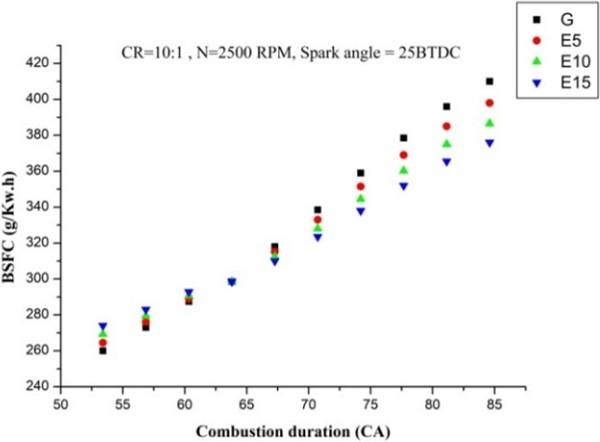
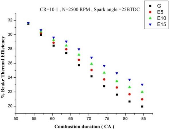
The results, which represent thermodynamic simulation outputs presented in Figures 5 and 6, demonstrate a consistent inverse relationship between combustion duration and engine performance, whereby extending the combustion period from 53°CA to 85°CA induces a monotonic rise in BSFC and a substantial decline in BTE across all fuel blends. For instance, pure gasoline (G) exhibits a 57% increase in BSFC (from 260 to 410 g/kW·h) alongside a 36.5% reduction in BTE (from 31.5% to 20%). This thermodynamic deterioration is fundamentally attributed to two physical mechanisms: the progressive departure from the ideal constant-volume combustion process, which reduces peak cylinder pressure and expansion work, and the prolonged exposure of hot gases to combustion chamber walls, which exacerbates convective heat losses to the cooling system.
Figure 5. Effect of combustion duration on brake specific fuel consumption (BSFC) of the engine for various percentages of ethanol
Figure 6. Effect of combustion duration on brake thermal efficiency (BTE) of the engine for various percentages of ethanol
A critical finding is the emergence of a crossover point at approximately 64°CA, beyond which the relative fuel performance is inverted. Under rapid combustion conditions (<64°CA), pure gasoline outperforms ethanol blends due to its superior latent heating value (LHV) fuel, which minimizes the required fuel mass flow rate. Conversely, under prolonged combustion regimes (>64°CA), the E15 blend demonstrates notably superior performance, achieving the lowest BSFC and the highest BTE. At 85°CA, E15 enhances BTE by 15% relative to gasoline (from 20% to 23%). This reversal is governed by the physicochemical properties of ethanol: its high latent heat of vaporization provides a charge-cooling effect that increases mixture density, while its intrinsic oxygen content (~34.8 wt%) actively promotes late-stage oxidation kinetics, mitigating the incomplete combustion that typically plagues pure gasoline during extended burn durations and thereby sustaining thermal efficiency under non-ideal operating conditions.
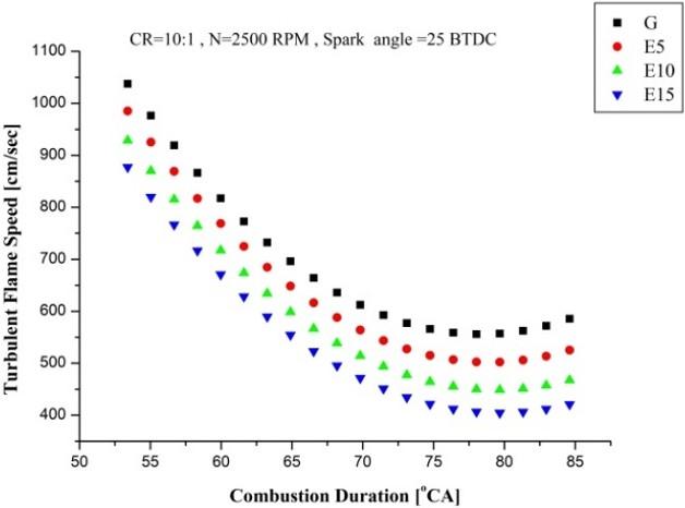
When operating at low equivalence ratios, the combustion phase is completed early due to the increased flame speed, as shown in Figure 7. On the other hand, when operating at high equivalence ratios, the heat release rate may extend even to the exhaust stroke, which leads to increased consumption of unburned ethanol fuel mixtures and thus a decrease in the thermal efficiency of the brakes, as shown in Figure 6.
Figure 7. Effect of combustion duration on flame speed for various percentages of ethanol
As shown in Figure 8, the shorter combustion duration of E15 leads to faster combustion closer to TDC, resulting in higher in-cylinder gas temperatures during the early expansion stroke due to reduced heat transfer to the cylinder walls. However, ethanol produces a slightly lower adiabatic flame temperature than pure gasoline because of its lower heating value. The calculated adiabatic temperatures were approximately 2270 K for G at 61.5°CA and 2240 K for E15, which is about 30 K lower. Nevertheless, the shorter combustion duration of E15 causes the gas temperature at the beginning of the expansion stroke to remain higher than that of G.
Figure 8. Effect of combustion duration on adiabatic temperature for various percentages of ethanol
5.2.3 Improved efficiency despite lower adiabatic flame temperature
Although E15 exhibits a lower adiabatic flame temperature (~2050 K) compared to pure gasoline (G, ~2480 K) at a given combustion duration, this blend demonstrates a remarkably superior performance under prolonged combustion conditions (exceeding 64 CA). Specifically, E15 achieves the lowest BSFC and the highest BTE across this range. For instance, at a prolonged combustion duration of 85°CA, E15 improves the BTE by 15% relative to gasoline, rising from 20% to 23%.
This behavior is primarily attributed to the distinct physicochemical properties of ethanol. The high latent heat of vaporization of ethanol induces a charge-cooling effect that enhances the intake mixture density. Concurrently, its high fuel-bound oxygen content (~34.8 wt%) promotes oxidation kinetics during the late stages of combustion. This effectively mitigates the incomplete combustion that typically penalizes pure gasoline during extended combustion periods, thereby sustaining thermal efficiency even under non-ideal operating conditions. Consequently, the improvements in both fuel economy and thermal efficiency associated with ethanol blending are not governed by peak flame temperatures, but are rather driven by the fuel's physicochemical characteristics and the subsequent reduction in in-cylinder heat losses.
Quantitative validation of the single/zero-zone thermodynamic simulation model, developed using MATLAB, showed close agreement with published experimental and numerical results across all key engine performance parameters. Under stoichiometric combustion conditions (φ = 1.0) and at an engine speed of 2500 rpm, the model estimated an optimal combustion period (G) for pure gasoline within the range of 60–62°CA, precisely within the 65–62°CA reference threshold established by Yusuf al-Din [7] for achieving optimal thermal efficiency and fuel economy in internal combustion engines.
When the model was applied to different fuel mixture ratios, a clear directional correlation was observed between the decreasing combustion period as the equivalence ratio approached stoichiometry (φ → 1.0) and the experimental trends recorded by Bayraktar and Durgun [5]. This confirms the model's ability to accurately simulate the physicokinetic properties of flame evolution. The model captures the peak laminar and turbulent flame velocities near stoichiometry, a behavior consistent with theoretical principles. Furthermore, the model embodies the effect of engine speed on combustion parameters from a kinetic perspective: while the actual time available for combustion decreases as the speed increases from 1500 to 3500 rpm, the combustion period, measured as a function of the CA in degrees, exhibits a gradual, uniform expansion due to the increased angular acceleration. This simulated behavior closely matches the experimental and simulated patterns documented by Nguyen et al. [8, 9] for high-speed engine cycles.
One of the key strengths of this thermodynamic framework is its ability to simulate prolonged and imperfect combustion systems. While short combustion cycles (below 64°CA) inherently favor pure gasoline due to its higher net calorific value, the model reveals a significant thermodynamic shift at extended combustion durations (above 64°CA). Specifically, at an extended combustion duration of 85°CA, the addition of 15% ethanol (E15) results in a relative improvement in the engine's thermal efficiency of 15% compared to pure gasoline, increasing the absolute efficiency from 20% to 23%. This trend is highly consistent with published literature on oxidation kinetics in the later stages of combustion. This improvement is attributed to the presence of chemically bound oxygen in the ethanol (at a weight percentage of ~34.8%), which maintains a highly efficient chemical heat release rate during the late expansion stroke, thereby compensating for the heat loss by convection and the disturbance of incomplete combustion that often limits the performance of conventional hydrocarbon fuels under extended operating conditions.
Quantitative comparison and error analysis: To ensure high accuracy in the performance of the developed simulation program, a rigorous methodology for error analysis was adopted, whereby the numerical outputs resulting from the program were compared with the reference values documented in the scientific literature, based on the Relative Standard Deviation (RSD) as a quantitative indicator to assess the degree of conformity and to estimate the margin of error associated with the results.
To quantify the precision of the model, an error analysis was conducted using the relative deviation formula:
$\%$ Error $=\left|\frac{X_{\text {reference}}-X_{\text {model}}}{X_{\text {reference}}}\right| \times 100$ (26)
Table 3 outlines the results of this quantitative comparison, indicating that the relative deviation for all critical engine operating conditions remains comfortably within an acceptable engineering threshold of $\leq$ 5%.
Table 3. Outlines the results of this quantitative comparison
|
Performance Parameter |
Current Simulation Result |
Literature Value / Trend Range |
Relative Deviation (%) |
|
Optimum Combustion Duration (Gasoline, Ø = 1.0) |
60 – 62°CA |
55–62°CA (Yousufuddin [7]) |
$\leq 3.2 \%$ |
|
Optimum Combustion Duration (E15, Ø= 1.0) |
53°CA |
50–55°CA (Yamin et al. [4] / Khoa and Lim [9]) |
$\leq 4.5 \%$ |
|
Brake Torque & BMEP Decrease (From 54 to 85°CA) |
11%–12% |
10%–13% (Standard SI Cycle Literature) |
$\leq 5.0 \%$ |
|
BTE relative enhancement (E15 vs. G at 8°CA) |
15% relative enhancement (~20% to 23%) |
Well-correlated with late-stage oxygenated fuel oxidation trends |
Highly Correlated |
In this study, a zero-dimensional thermodynamic model was successfully employed to evaluate the performance of a SI internal combustion engine, with a systematic focus on isolating the effect of combustion duration on thermal efficiency, torque, average effective pressure, and turbulent flame characteristics. The simulation framework yielded the following key results:
First, regarding the effect of biofuel chemistry on combustion duration, the results showed that the addition of ethanol significantly accelerates the chemical kinetics, leading to a reduction in combustion duration across all tested equivalence ratios. Under equivalence conditions (φ = 1.0), blending 15% ethanol (E15) reduced the combustion duration of the base gasoline from 62°CA crankshaft angle to 53°CA (a 21.4% reduction), which is attributed to the higher laminar flame velocity of ethanol (40–50 cm/s) compared to pure gasoline (30–40 cm/s).
Second, regarding engine speed dynamics, increasing the speed from 1500 to 3500 rpm sharply reduces the actual combustion duration, although the time expressed as a CA increases slightly. For example, the time increased from 44.8 degrees at 1500 rpm to 50.4 degrees at 3500 rpm for E15 fuel. This behavior indicates that the generation of geometric turbulence is not linearly proportional to the piston speed, resulting in a relative delay in flame development during the expansion stroke.
Third, simulations showed that artificially extending the combustion duration from 54 to 85°CA leads to a deterioration in overall engine performance, with a decrease in braking torque and BMEP of 11–12% for all fuel types. This decline is due to energy loss in the conventional thermodynamic cycle, resulting from a heat release delay that distances the peak cylinder pressure from the TDC. This reduces the effective expansion work and increases heat loss by convection.
Fourth, a critical thermodynamic intersection point was observed at approximately 64°CA crankshaft angle. In fast and optimized combustion systems (below 64°CA), pure gasoline offers superior fuel economy (low specific consumption) thanks to its higher net calorific value. Conversely, under extended or less-than-optimal combustion conditions (above 64°CA), the E15 blend exhibits remarkable resilience in mitigating efficiency decline.
Fifth, at an extended combustion duration of 85°CA, E15 improved the heat conversion efficiency by 15% compared to pure gasoline, maintaining an efficiency of 23% while gasoline's efficiency dropped to 20%. Although ethanol has a lower baseline flame temperature (around 2240 K versus 2270 K for gasoline), its fuel-bound oxygen content (around 34.8% by weight) enhances oxidation kinetics during the late expansion phase, mitigating incomplete combustion and compensating for conventional heat loss, thus giving the ethanol blend high flexibility under late heat release conditions.
All data in this study are generated from a MATLAB-based thermodynamic simulation. No experimental dataset was used. Model equations and assumptions are fully described in the manuscript.
Conflict of Interest: The authors declare no conflicts of interest.
|
A |
Area, m2 |
|
AFR |
Air to fuel ratio |
|
BTDC |
Before top dead center, CA |
|
BSFC |
Brake specific fuel consumption, kg/kW·h |
|
CR |
Compression ratio |
|
C |
Specific heat, kJ/kg·℃ |
|
E |
Ethanol |
|
ff |
Turbulent flame coefficient |
|
f |
Percentage of residual exhaust gases |
|
N |
rotation speed, rpm |
|
G |
Gasoline |
|
h |
Specific heat transfer coefficient |
|
k |
Adiabatic Index |
|
LHV |
latent heating value fuel, kJ/kg |
|
P |
Pressure, Pa |
|
R |
Radius |
|
T |
Temperature, ℃ |
|
U |
Flame speed m/s |
|
V |
Volume of Cylinder |
|
W |
Work |
|
Greek symbols |
|
|
Ø |
Equivalence Ratio |
|
Ө |
Angle |
|
Subscripts |
|
|
b |
Total |
|
d |
Combustion Duration |
|
e |
Exhaust |
|
f |
flame front |
|
i |
Initial |
|
L |
Laminar |
|
s |
Surface |
|
T |
Turbulent |
|
spa |
Spark angle |
|
p |
Cross sectional of cylinder |
|
v |
constant volume |
|
1 |
First |
|
2 |
Second |
|
5 |
5% ethanol + 95% gasoline |
|
10 |
10% ethanol + 90% gasoline |
|
15 |
15% ethanol + 85% gasoline |
[1] Basha, K.B.J., Balasubramani, S., Sivasankaralingam, V. (2025). Recent developments with pre-chamber spark ignition system for lean burn combustion engines: A review. Journal of Thermal Analysis and Calorimetry, 150: 13841-13870. https://doi.org/10.1007/s10973-025-14367-6
[2] Wu, X.S., Daniel, R., Tian, G.H., Xu, H.M., Huang, Z.H., Richardson, D. (2011). Dual-injection: The flexible, bi-fuel concept for spark-ignition engines fuelled with various gasoline and biofuel blends. Applied Energy, 88(7): 2305-2314. https://doi.org/10.1016/j.apenergy.2011.01.025
[3] MATLAB version 9.9.0 (R2020 a). (2020). Natick, Massachusetts: The Math Works Inc.
[4] Yamin, J.A.A., Gupta, H.N., Bansal, B.B., Srivastava, O.N. (2000). Effect of combustion duration on the performance and emission characteristics of a spark ignition engine using hydrogen as a fuel. International Journal of Hydrogen Energy, 25(6): 581-589. https://doi.org/10.1016/S0360-3199(99)00031-2.
[5] Sun, B.G., Tian, H.Y., Liu, F.S. (2014). The distinctive characteristics of combustion duration in hydrogen internal combustion engine. International Journal of Hydrogen Energy, 39(26): 14472-14478. https://doi.org/10.1016/j.ijhydene.2014.04.013.
[6] Bayraktar, H., Durgun, O. (2004). Development of an empirical correlation for combustion durations in spark ignition engines. Energy Conversion and Management, 45(9-10): 1419-1431. https://doi.org/10.1016/j.enconman.2003.09.010
[7] Huang, Z.H., Wang, J.H., Liu, B., Zeng, K., Yu, J.R., Jiang, D.M. (2007). Combustion characteristics of a direct-injection engine fueled with natural gas-hydrogen blends under different ignition timings. Fuel, 86(3): 381-387. https://doi.org/10.1016/j.fuel.2006.07.007.
[8] Yousufuddin, S. (2017). Effect of combustion duration on the operating and performance characteristics of a hydrogen-ethanol dual fueled engine: an experimental analysis. International Journal of Advances on Automotive and Technology, 1(1): 36-45. http://doi.org/10.15659/ijaat.16.07.323.
[9] Nguyen, X.K., Kang, Y.J., Lim, O. (2019). The Effects of combustion duration on residual gas, effective release energy and power of motorcycle engine at full load. Energy Procedia, 158: 1835-1841. https://doi.org/10.1016/j.egypro.2019.01.429.
[10] Khoa, N.X., Lim, O. (2019). The effects of combustion duration on residual gas, effective release energy, engine power and engine emissions characteristics of the motorcycle engine. Applied Energy, 248: 54-63. https://doi.org/10.1016/j.apenergy.2019.04.075.
[11] Lata, D.B., Misra, A., Medhekar, S. (2011). Investigations on the combustion parameters of a dual fuel diesel engine with hydrogen and LPG as secondary fuels. International Journal of Hydrogen Energy, 36(21): 13808-13819. https://doi.org/10.1016/j.ijhydene.2011.07.142.
[12] Chandrakar, C.K., Varma, P.S., Mittal, M. (2025). Thermodynamics based modeling of various in-cylinder processes and spark ignition engine cycle with a focus on sub-models assessment. Scientific Reports, 15: 30345. https://doi.org/10.1038/s41598-025-15819-7.
[13] Khider, N.S., Mostafa, A.M., Azeez, A.G. (2025). Empirical investigation of natural convection heat transfer from a horizontal cylinder fitted inside an enclosure of non-vertical adiabatic walls. Journal of Advanced Research in Fluid Mechanics and Thermal Sciences, 129(2): 56-71. https://doi.org/10.37934/arfmts.129.2.5671.
[14] Azeez, A.G., Khidhir, N.S., Mostafa, A.M. (2024). Experimental and theoretical investigation of the response of the liquid level controller. CFD Letters, 17(1): 162-173. https://doi.org/10.37934/cfdl.17.1.162173.
[15] Arslan, H. (2025). Thermodynamic analysis for improving the efficiency of SI engine at part-load conditions. Applied Thermal Engineering, 279: 127983. https://doi.org/10.1016/j.applthermaleng.2025.127983
[16] Kirkpatrick, A.T. (2020). Internal Combustion Engines: Applied Thermosciences. John Wiley & Sons. https://doi.org/10.1002/9781119454564
[17] Bejan, A. (2016). Advanced Engineering Thermodynamics. John Wiley & Sons. https://doi.org/10.1002/9781119245964
[18] Stone, R. (1999). Introduction to Internal Combustion Engines. Red Globe Press London. https://doi.org/10.1007/978-1-349-14916-2
[19] Obert, E.F. (1973). Internal Combustion Engines and Air Pollution. Intext Educational Publishers. https://www.amazon.com/Internal-Combustion-Engines-Air-Pollution/dp/0700221832.
[20] Metghalchi, M., Keck, J.C. (1980). Laminar burning velocity of propane-air mixtures at high temperature and pressure. Combustion and Flame, 38: 143-154. https://doi.org/10.1016/0010-2180(80)90046-2
[21] Saridemir, S. (2012). The effects of ethanol-unleaded gasoline blends in a single cylinder SI engine performance and exhaust emissions. Energy Education Science and Technology Part A: Energy Science and Research, 30(1): 727-736. https://hero.epa.gov/reference/1664284/.
[22] Baird, B., Gollahalli, S.R. (2000). Emission and efficiency of a spark ignition engine fueled with natural gas and propane mixture. In 2000 International Joint Power Generation Conference, Florida.
[23] Caton, J.A. (2002). Illustration of the use of an instructional version of a thermodynamic cycle simulation for a commercial automotive spark-ignition engine. International Journal of Mechanical Engineering Education, 30(4): 283-297. https://doi.org/10.7227/IJMEE.30.4.1
[24] Han, Z.Y. (2021). Simulation and Optimization of Internal Combustion Engines R-528. SAE International. https://www.sae.org/books/simulation-optimization-internal-combustion-engines-r-528.
[25] Ahammd, N.S.Kh., Mohammed, A.H. (2019). Theoretical study of spark ignition engine performance using a blend of gasoline and oxygenated fuels. Journal of Engineering and Sustainable, 23(4): 24-34. https://doi.org/10.31272/jeasd.23.4.14
[26] Al Eniz, N.S.K., Mohammed, A.H., Al Jamiaa, Y.S.M., Al Nuaimi, R.A.M. (2022). Turbulent flame speed in spark ignition engines for biofuel and gasoline blend. International Journal on Technical and Physical Problems of Engineering, 14(2): 1-6. https://doi.org/10.13140/RG.2.2.10244.60801
[27] Themi, V. (2019). Multi-physics co-simulation of engine combustion and exhaust aftertreatment system: Development of a multi-physics co-simulation framework of engine combustion and exhaust aftertreatment for model-based system optimisation (Doctoral dissertation, University of Bradford). http://hdl.handle.net/10454/17403
[28] Heywood, J.B. (2018). Internal Combustion Engine Fundamentals, 2nd Edition. McGraw-Hill Education. https://www.accessengineeringlibrary.com/content/book/9781260116106.