Hussein M. Al-Mrayatee![]()
© 2025 The author. This article is published by IIETA and is licensed under the CC BY 4.0 license (http://creativecommons.org/licenses/by/4.0/).
OPEN ACCESS
A numerical study of a proposed dual-zone liquid metal reactor (DZLMR) for CO2 capture by a redox-based chemical looping approach. The coupled governing equations for mass and energy transport are coupled with temperature dependent reaction kinetics and solved to access the possibility and optimization of the dual-zone configuration. Various pertinent process parameters such as the inlet gas temperature, reactive metal concentration, flow velocity, reactor length, etc., were systematically changed to investigate the influence of these on the CO2 conversion efficiency. The results show that CO2 conversion increased from 43.5% to 58.2% with an increase in the inlet temperature from 800 K to 1000 K. Also raising the metal concentration from 2.0 mol/m3 up to 3.0 mol/m3 improved the conversion to 52.7%. Decreasing flow velocity from 0.005 m/s to 0.002 m/s increased gas–metal interaction time, resulting in 61.3% of conversion. Reaction product conversion increased dramatically from 32.1% to 62.8% on increasing the reactor length from 0.5 m to 1.5 m. These results underscore the significance of both, thermal zoning and reactor design on the system performance. The dual-zone strategy provides improved regulation of heat transfer and reaction paths, thus proving highly applicable in energy consuming sectors such as power, cements and metals production. The inferences that can be drawn from literature data provide a basis for practical optimization of scalable, high-efficiency CO2-sequestration technology.
CO2 capture, dual-zone reactor, liquid metal, chemical looping, mass and energy transport, reaction kinetics, numerical simulation, metal oxide redox, temperature gradient, reactor optimization
There has been an urgent drive to capture and use CO2 because of the need to reduce global emissions, causing the growth of new technologies. Because of their high thermal conductivity, strong chemical stability and quick gas-absorbing properties, reactors that use liquid metal as their medium have attracted increased interest. One particular example is the use of dual-zone liquid metal reactors (DZLMRs) to make the best use of temperature differences in space for better carbon dioxide absorption and regeneration. Having dual zones allows separating the CO2 absorption zone and the regeneration zone, usually setting one area at a higher temperature and the other at a lower temperature. Dividing the process in this way enhances the control of chemical reaction and improves chemical looping and reforming when using metal oxides or catalytic surfaces in the liquid metal chamber. Using numerical methods and CFD as well as other solvers is now required to study and understand the complex processes of energy and matter movement in DZLMRs. They let researchers visualize internal flow details, estimate temperature patterns and study the reactions occurring between gas and metal in practical operating conditions. Fix-bed and packed reactors have had a lot of research, but the simulation of dual-zone liquid metal systems is not yet well explored. Work reported in literatures on chemical looping, solar thermochemical conversion and high-flux catalytic reformers provides useful basics but does not directly tackle coupled transport in DZLMRs. The purpose of the study is to fill this gap by showing a detailed simulation of energy and mass flows in a liquid metal reactor suited for CO2 capture. The main aim is to check how heat transfer, air movement and CO2 absorption vary between the two zones. As a result, this work plays a part in improving carbon capture technologies for the next stage that are efficient and capable of mass production.
De Wilde and Froment [1] designed a Computational Fluid Dynamics (CFD) model for steam reforming of natural gas in dual-zone reactors. They explained why combining detailed description of fluid flows in the pores with less-detailed near-wall description helps to improve the transport of heat and mass in dual-zone systems that is very relevant for DZLMRs managing CO2. Battani et al. [2] detailed it that metal oxides can be used as oxygen carriers in the process of converting CO2 and reforming it. Researchers have covered the thermodynamics of reactors and mass transfer mechanisms which are especially useful for DZLMRs based on metals. Zhang et al. [3] looked into designs of advanced heat exchangers/reactors that hold liquid metals, placing importance on maintaining proper temperature differences due to thermal inertia found in the reactor walls. Mateo et al. [4] introduced Photothermal catalysis to join light and heat into one method. What they learned on nanostructured catalysts and plasmonic materials can be used to make thermal distribution and CO2 reduction better in photothermally-driven DZLMRs. Suyadal [5] discussed methane reforming in fluidized beds and compared it to bubble motion and resistance to mass transfer, both of which must be controlled well in reactors that include bubbles and fluidized particles. Mandal et al. [6] found a close connection between mass transport limits, catalyst surface area and porosity for thermo-catalytic biomass conversion which plays a key role when simulating DZLMR under varying temperatures. Roos [7] explained in detail how important factors for biomass gasification systems, like heat transfer problems, fouling and slagging, can affect the simulation accuracy of reactor designs for capturing CO2 using any type of tubing or wall lining. A study in Applied Energy studied chemical looping combustion using molten metal oxides [8]. The study looked at redox cycles and the rates at which oxygen is transferred in a DZLMR. Today’s catalytic reformers and their layered design stress controlling the core-casing permeability and turbulence which has led to more accurate simulation in divided reactors [9]. The team of Cui et al. [10] examined the difficulties of scaling up and defined new performance metrics for photothermal systems. Using similar ways they use to measure thermal gradients and enhance photon absorption, DZLMRs active in solar-assisted CO2 reforming can be improved.
It was mentioned by Hamzah et al. [11] that better heat and mass transfer can be achieved in microreactors by using structures which supports the idea of dual-zone configurations using temperature differences to improve chemical reforming. Also, Brkic [12] studied solar-powered drop-tube reactors for thermochemical reduction, finding that temperature differences through the reactor and the time materials remain inside it are important for reaction speed and flow of the substances. Cameron et al. [13] explained how numerical simulations play a key part in understanding gas–solid contact within loop reactors by giving advice on how to optimize liquid metal flow and CO2 interactions with CFD. According to Li et al. [14], a multi-zone simulation model for chemical looping combustion (CLC) was developed, confirming that compartmental reactors aid in better conversion of carbon in the process. Ramos-Fernandez et al. [15] present an example of using thermal and photonic control in catalysts which can efficiently boost energy conversion in areas such as high-temperature CO2 reactors with liquid metals. Leon et al. [16] showed the importance of proper reactor design by running gasification experiments under various transport conditions and temperature differences. According to Xu et al. [17] chemical looping’s main focus is producing synthesis gas and she showed that oxygen carriers and related processes cannot be overlooked, a factor that matches aspects of mass transport phenomena involved in DZLMR operations with reactive liquid metals. Loureiro et al. [18] discussed experiments with metal-based reactors to study the behavior of liquid metal in dual zones. Hogan et al. [19] published one of the earliest studies on integrating biological biofiltration with heating and cooling, whose concept is closely matched by recent work on integrated heat and mass transport. On top of that, Robles-Lorite et al. [20] gave a step-by-step process to numerically study catalytic systems, pointing out that the way the substrates are shaped and the transport of materials within the reactor are vital for designing dual-zone reactors.
They found from ion exchange studies in zeolite-based molten salts [21] that the direction and mobility of charged particles inside porous crystals are affected by internal diffusion. Even though dechlorination processes are mainly discussed, the findings suit CO2 removal using liquid metals with significant surface interaction and selectivity. Thompson and Kwon [22] tested how different pressure and fluid ratio ratios affected how efficiently a fluid can be displaced in dual-zone porous media. The way they build their model guarantees a match with the dual-reactor strategy for capturing CO2, particularly when studies areas where selective displacement zones are considered. CFD simulation of monolithic micro-circulating bed reactors in the TC-QQLA study helped understand how gas-solid interactions in tiny channels lead to different levels of conversion [23]. It is much like creating interface surfaces for gasses, liquids and metals in high-temperature spots for CO2 absorption technologies. Betar et al. [24] highlighted that using symmetry and thermodynamic boundaries can improve how multi-zone reactors work and how their flows are controlled. Their scheme may be modified to enhance temperature zones in a DZLMR. Jia et al. [25] suggested a liquid-metal-assisted thermal management system for reforming reactions because liquid metals offer strong conductivity and uniformity—both of which are important in CO2 capture systems.
The worldwide urgency of limitation of the greenhouse gas emission has increased towards a deep investigation of an efficient carbon capture. Among these, liquid metal reactors have been highlighted because of their remarkable thermal conductivity, chemical stability as well as perfect gas–metal interaction performance. However, the majority of previous studies have concentrated on single-zone and packed-bed systems which do not provide accurate control of the spatial distribution of temperature and reaction pathways. To overcome these limitations, in this study, the design of a Dual-Zone Liquid Metal Reactor (DZLMR) is proposed and performance is discussed through analyzing the CO2 capture and release process in two different zones of the reactor. This decoupling offers superior reaction control and efficiency by optimal thermal management. Although the literature previously studied chemical looping or molten metal systems for the CO2 reforming or syngas generation, in general they failed to combine a fully couple simulation of mass and energy transport simultaneously into the dual-zone system. The novelty of the paper is the integrated 1D model that accounts for the coupled transport phenomena and reaction kinetics throughout the two zones, describing the dynamic behavior of reactive metal cycling, gas flow and temperature gradients. Changing the inlet temperature, reactor length, gas velocity, and metal concentration, the model offers an interpretation of how the dual zone design can be optimized in terms of CO2 conversion. This will provide not only a fundamental understanding about the multi-zone metal reactor, but will also lead to a viable, scalable, high-efficiency platform that can be incorporated into energy-demanding industrial processes. Accordingly, the present study fills a significant gap in the literature by integrating innovative reactor design with detailed simulations towards furthering carbon capture technology.
The focus of this study is to design and model a DZLMR for cost-effective CO2 capture using redox-based chemical looping. The simulation is developed in order to examine the effects of vital process parameters, loose packed bed inlet temperature, reactor length, gas flow rate and reactive metal content on energy and mass transfer, chemical kinetic and overall CO2 conversion efficiency. By considering these effects in a dynamic numerical model, the study attempts to determine the operating conditions at which carbon sequestration is maximized and steady reactor operation is successfully maintained. Apart from its theoretical importance, it can be directly applied to the energy expenditure in industry driven processes, such as power, cement, steel and chemical production that are among the biggest CO2 emitters in the world. Due to its modular structure with separated absorption and regeneration zones, the DZLMR can be scaled and tailored for integration with retrofits to existing industrial systems. Its capacity to cope with high thermal loads and the ease with which it can regenerate the reactive materials makes it an attractive candidate for future systems that must possess not only performance but also flexibility.
The originality of this work is to build and utilize a coupled mass–energy transport simulation tool for a DZLMR, specifically designed in order to be coupled with a high efficiency CO2 capture system. In contrast to prior studies that are usually limited to single-zone designs, packed beds, or simplified thermal models, this study couples spatially resolved transport dynamics, reaction kinetics, and temperature-dependent phenomena across the oxidation and regeneration zones. This split-bed separation facilitates thermally efficient chemical looping with control of both the endothermic and exothermic reactions independently, a key requirement for industrial relevance but one that has been largely uninvestigated in the literature. Furthermore, the reactor model is not only theoretically sound but also readily transferable to practical industrial processes like steel production, cement production, and thermopower plants, where CO2 emissions are high and where temperature gradients are integral to the process. Through modeling of various scenarios with parameters such as inlet temperature, velocity and metal concentration, the work gives a useful tool to engineers for designing and operating of the next generation of CO2 capture technology. Specifically, this work fills a critical knowledge gap by revealing how a modular dual-zone reactor design can be optimized for increased gas conversion and energy capture, furthering both fundamental knowledge and deployment readiness.
2.1 Reactor configuration and working mechanism
Trials are being done in a dual-zone liquid metal reactor to produce both syngas and slow down CO2 emissions by using a reactive metal (M). The capture-conversion cycle depends on the two main zones in the reactor which are called the oxidation zone and the regeneration zone.
During the first section of the reactor (oxidation zone), carbon dioxide and water from the input gas mix with a reactive metal surface. Exothermic reactions happen in two important parts of the process:
$\mathrm{CO}_2+\mathrm{M} \rightarrow \mathrm{MCO}_2$ (1)
$\mathrm{H}_2 \mathrm{O}+\mathrm{M} \rightarrow \mathrm{H}_2+\mathrm{MCO}_2$ (2)
These reactions serve to capture CO2 while simultaneously generating hydrogen (H2), an essential component of syngas. As these reactions proceed, the concentration of the reactive metal decreases due to its transformation into a metal carbonate intermediate (MCO2).
In the second half (regeneration zone), the previously formed MCO2 undergoes an endothermic decomposition reaction:
$\mathrm{MCO}_2 \rightarrow \mathrm{M}+\mathrm{CO}$ (3)
The metal is regenerated in this step and carbon monoxide (CO) is produced which finishes the creation of syngas. The metal can be used repeatedly to keep capturing CO2 in a circular manner. The reactor is considered to be a one-dimensional flow where temperature, species amounts and reaction rates change from one end to the other. Mass transport, energy transfer and chemical kinetics are all joined in the framework to mimic the actual operation while showing the main dynamics of CO2 capture and utilization.
2.2 Operating conditions and initial parameters
Operating conditions were set up carefully to examine the thermal and chemical effects within the simulation of the dual-zone liquid metal reactor. Reactor lengths were varied between different tests (0.5, 1 and 1.5 m) to see how the reactor’s size influenced its performance. 200 evenly spaced elements represented the space inside the reactor, with time advancing every 0.002 seconds until the simulation reached 10 seconds, so both the space and time were well represented. The base temperature of the inlet was fixed at 800 K, but variations were considered later to test how sensitivity changes. Here, the word “defined” describes the way in which the quantities of the first gases were established:
$\begin{gathered}\mathrm{CO}_2: 1.0 \mathrm{~mol} / \mathrm{m}^3 \\ \mathrm{H}_2 \mathrm{O}: 0.5 \mathrm{~mol} / \mathrm{m}^3\end{gathered}$
CO and $\mathrm{H}_2: 0 \mathrm{~mol} / \mathrm{m}^3$ (not present at inlet).
$\mathrm{MCO}_2: 0 \mathrm{~mol} / \mathrm{m}^3$ (formed in situ).
Reactive Metal (M): linearly decreasing from $2.0 \mathrm{~mol} / \mathrm{m}^3$ at the inlet to $0.5 \mathrm{~mol} / \mathrm{m}^3$ at the outlet, representing a higher metal presence in the oxidation zone.
To match the different residence times in different zones, the stationary part of the flow was first stepped down to 0.003 m/s and after that raised to 0.005 m/s in the second zone.
Empirical correlations were created to model the thermal conductivity and specific heat capacity that depend on the temperature:
$c_p(T)=140+0.05 \cdot T[\mathrm{~J} / \mathrm{kg} \cdot \mathrm{K}]$ (4)
$k(T)=25+0.02 \cdot T[\mathrm{~W} / \mathrm{m} \cdot \mathrm{K}]$ (5)
Using these inputs, the reactor model correctly simulates all energy, mass and chemical reactions during the reactor’s entire operational cycle.
2.3 Reaction kinetics and pathways
This kind of reactor works thanks to a succession of chemical reactions that allow CO2 capture and also produce syngas by using metals. The rate at which these reactions happen is controlled by the Arrhenius law that changes with temperature. There are three chemical reactions in the model and each reaction has particular kinetic parameters:
1. CO2 Reduction (Oxidation Zone)
Reaction: $\mathrm{CO}_2+\mathrm{M} \rightarrow \mathrm{MCO}_2$
Type: Exothermic
Kinetics: $R_1=A_1 \cdot\left[\mathrm{CO}_2\right]^{1.1} \cdot[\mathrm{M}]^{0.9} \cdot \exp \left(\frac{-E_{\mathrm{at}}}{I T T}\right)$
Parameters: $A_1=2000 \mathrm{~s}^{-1}, E_{a 1}-60,000 \mathrm{~J} / \mathrm{mol}, \Delta H_1= -300,000 \mathrm{~J} / \mathrm{mol}$
2. H2O Reduction (Oxidation Zone)
Reaction: $\mathrm{H}_2 \mathrm{O}+\mathrm{M} \rightarrow \mathrm{H}_2+\mathrm{MCO}_2$
Type: Exothermic
Kinetics: $R_2=A_2 \cdot\left[\mathrm{H}_2 \mathrm{O}\right]^{1.2} \cdot[\mathrm{M}]^{0.8} \cdot \exp \left(\frac{-E_{01}}{I T T}\right)$
Parameters: $A_2=500 \mathrm{~s}^{-1}, E_{a 2}-\frac{70,000 \mathrm{~J}}{\mathrm{~mol}}, \Delta H_2=-150,000 \mathrm{~J} / \mathrm{mol}$
3. Metal Regeneration (Regeneration Zone)
Reaction: $\mathrm{MCO}_2 \rightarrow \mathrm{M}+\mathrm{CO}$
Type: Endothermic
Kinetics: $R_3=A_3 \cdot\left[\mathrm{MCO}_2\right]^{1.3} \cdot \exp \left(\frac{-E_{\mathrm{an}}}{I T T}\right)$
Parameters: $A_3=1000 \mathrm{~s}^{-1}, E_{a 3}-\frac{80,000 \mathrm{~J}}{\mathrm{~mol}}, \Delta H_3=+200,000 \mathrm{~J} / \mathrm{mol}$
All reactions change the chemical composition and influence the reactor’s use of energy using chemical reaction enthalpies. A constant process requires both CO2 capture and metal regeneration to be kept in balance between these two zones. Besides, kinetics are adjusted with a temperature correction factor (1+0.001⋅T) to better reflect the faster reactions that happen at higher temperatures.
Kinetic expressions are added to the conservation equations, so the simulation can track how the reactions develop over time and distance in the reactor.
2.4 Governing equations for mass and energy transport
The simulation of a dual-zone liquid metal reactor involves both mass and energy conservation, which outlines the way the concentration, and temperature changes along the reactor. It is assumed that the flow is steady, continuous and one-way and does not take into account small side-to-side mixing also, this model considers bulk transport rather than molecular diffusion.
2.4.1 Mass conservation equations
The mass balance for each chemical species incorporates convective transport and reaction source terms. For a generic species Ci, the mass conservation equation is written as:
$\frac{\partial C_i}{\partial t}+u \frac{\partial C_i}{\partial z}=R_i$ (6)
where:
$C_i$: Concentration of species $i\left[\mathrm{~mol} / \mathrm{m}^3\right]$
$u$: Axial velocity profile $[\mathrm{m} / \mathrm{s}]$
$z$: Axial position along the reactor [ m ]
$R_i$: Net reaction rate for species $i\left[\mathrm{~mol} /\left(\mathrm{m}^3 \cdot \mathrm{~s}\right)\right]$
The reaction terms Ri differ for each species, depending on their participation in the three main chemical reactions (R1, R2, R3), as previously defined in the kinetics section.
2.4.2 Energy conservation equation
The energy balance considers convective heat transfer, axial conduction, and heat effects from chemical reactions. The equation governing the temperature T(z, t) is expressed as:
$\frac{\partial T}{\partial t}+u \frac{\partial T}{\partial z}=\alpha \frac{\partial^2 T}{\partial z^2}+\frac{1}{\rho c_p} Q_{\mathrm{rxn}}$ (7)
where:
$\alpha=\frac{k}{\rho c_p}$: Thermal diffusivity $\left[m^2 / s\right]$
$k$: Thermal conductivity $[W / m \cdot K]$, temperaturedependent
$c_p$: Specific heat capacity $[. \mathrm{J} / \mathrm{kg} \cdot \mathrm{K}]$, temperaturedependent
$\rho$: Density of the reactor medium $\left[\mathrm{kg} / \mathrm{m}^3\right]$
$Q_{\mathrm{rxn}}$: Total heat generated or absorbed by chemical reactions:
$Q_{\mathrm{rxn}}=\Delta H_1 R_1+\Delta H_2 R_2+\Delta H_3 R_3$ (8)
This formulation allows simulation of temperature variations resulting from reaction exothermicity and endothermicity, with heat accumulation and loss reflected in the spatial temperature distribution.
2.4.3 Numerical implementation
Finite differences are used to solve the partial differential equations that involve mass and energy.
• Solution in forward Euler’s step
Upwind method is the appropriate way to calculate convective terms.
• Fick’s law solved with central differencing (in the energy equation)
They are efficient and work reliably when the chosen time step and spatial resolution are respected. The approach gives a solid structure for tracking the influence of flow, heat and reactions in the reactor during the simulation.
2.5 Numerical implementation and boundary conditions
The reactor model is solved as a two-zone system by using a finite difference method in MATLAB, solving the linked mass and energy conservation equations as the liquid moves over space and time. In one spatial dimension, the domain is formed by dividing the reactor’s length into uniform intervals. It follows the changes in species numbers and temperature over time as operating conditions are changed.
2.5.1 Discretization scheme
Spatial Discretization: The reactor length $L$ is divided into $n$ equally spaced grid points with spacing $\Delta z-L / n$.
Time Discretization: A forward Euler method is applied for time integration with a time step $\Delta t$, iterating up to a final time $t_{\text {end }}$.
Convective Terms: Treated using an upwind finite difference to ensure numerical stability:
$\left.\frac{\partial C_i}{\partial z}\right|_j \approx \frac{C_i(j)-C_i(j-1)}{\Delta z}$ (9)
Diffusive Terms (only in the energy equation): Approximated using central differences:
$\left.\frac{\partial^2 T}{\partial z^2}\right|_j \approx \frac{T(j+1)-2 T(j)+T(j-1)}{\Delta z^2}$ (10)
2.5.2 Boundary conditions
To simulate a continuous flow reactor, appropriate boundary conditions are applied at the inlet ($z-0$) and outlet ($z-L$):
$\begin{gathered}C_{\mathrm{CO}_2}(1)-1.0 \mathrm{~mol} / \mathrm{m}^3, C_{\mathrm{H}_2 \mathrm{O}}(1)-0.5 \mathrm{~mol} / \mathrm{m}^3 \\ C_{\mathrm{CO}}(1)-0, C_{\mathrm{H}_2}(1)-0, C_{\mathrm{MCO}}(1)-0, C_{\mathrm{M}}(1)-2.0\end{gathered}$
2.5.3 Stability considerations
The choice of small time step $\Delta t=0.002 \mathrm{~s}$ ensures numerical stability, especially given the nonlinear nature of the reaction rates and the coupling with the energy balance. Temperature-dependent material properties and reaction rates further emphasize the need for a fine resolution in both time and space.
2.5.4 Code modularity
Because MATLAB code is modular, it is easy to change or expand its parts.
Because of this flexibility, parametric studies can be made on reactor behavior under changing design and operation conditions, as shown in the results and discussion section.
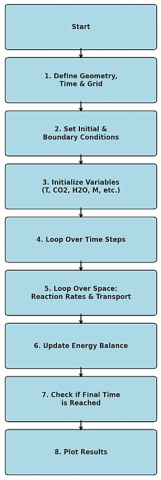
The reactor model combines mass/energy transport with temperature-dependent, kinetics modeling for the chemical reactions, within a one-dimensional simulation structure. They key parameters are chosen based on the theoretical basis and empirical precedent. The temperature interval (800 K to 1000 K) corresponds to common operating ranges for redox based CO2 capture with metal oxides, as demonstrated in recent works on molten metal chemical looping systems Majumdar et al. [9]; Minette and De Wilde [8]. This interval is broad enough to enable both strong exothermic CO2/H2O reduction and endothermic regeneration reactions without material stability of the reactors being impaired. The reaction kinetics are represented as Arrhenius-type expressions with temperature correction factors, and the activation energies and pre-exponential factors were selected to be consistent with those reported in other similar high-temperature gas–solid or gas–liquid metal systems Cameron et al. [13]; Mandal et al. [6]. The correspondence of conversion rates and length of reaction zones (physical) predicted with these parameters was also adjusted. Secondly, residence time and flow velocity (0.003–0.007) m/s values were chosen for considering realistic ranges utilized in industrial-scale reactors and for obtaining relevant simulation results so that they could be directly adopted for the purposes of process intensification and scale-up. For subsequent studies, these assumptions could be validated or modified based on experimental tuning, but here they provide a reasonable initial set of assumptions that give a compromise between computational tractability and practical operating conditions. Figure 1 show the process flow diagram of dual-zone liquid metal reactor simulation illustrating 1D coupled energy-mass transport and temperature-dependent kinetics for CO2 reforming.
Figure 1. Process flow diagram of dual-zone liquid metal reactor simulation illustrating 1D coupled energy-mass transport and temperature-dependent kinetics for CO2 reforming
Here, the results from a dual-zone liquid metal reactor are described and explored as a solution for CO2 capture and syngas production. For evaluation, the reactor performance was reported for changes in reactor length, temperature at the beginning of reaction, how fast the reactant flowed and the reactive metal concentration. The main aim is to study how these variables shape the transport of energy and materials, control chemical reactions and alter the number and types of species as the reaction progresses in the reactor. Each figure in this section highlights the pattern of important parameters such as temperature, gas concentrations (CO2, CO, H2O, H2, MCO2 and M) and CO2 conversion efficiency, across the reactor. Every figure demonstrates how CO2 utilization and hydrogen/carbon monoxide production depend on the choices made in reactor design. The study helps identify how to increase gas conversion, recover metals and handle energy more effectively in a reactor.
3.1 Effect of inlet temperature on energy and CO2 capture performance
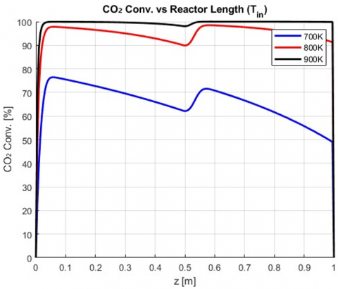
In Figure 2, see the portion of CO2 converted over the entire reactor (z=0 to 1 m) for temperatures of 700 K, 800 K and 900 K. Because the input at the reactor inlet z=0 m is pure CO2, its conversion rate is initially 0%. Since metal-aided processes happen, the conversion rises as the fuel passes through the reactor. The maximum increase in the fluid’s temperature reaches 82% for the 900 K pairing, compared to 70% for 800 K and 55% at 700 K. This trend demonstrates that heating the system speeds up the reactions, mainly for endothermic cases which is better for turning CO2 into fuel. The more dramatic conversion rate chart at 900 K indicates that early reactor zones experience faster start and completion of chemical reactions. In fact, the buildup of reaction products and limited access to reagents close to the reactor cause equilibrium and reactant depletion. It points out that setting the correct inlet temperature helps improve capture without causing major losses or deterioration.
Figure 2. Effect of inlet temperature (700–900 K) on CO2 conversion along the reactor length showing enhanced conversion kinetics at higher thermal input
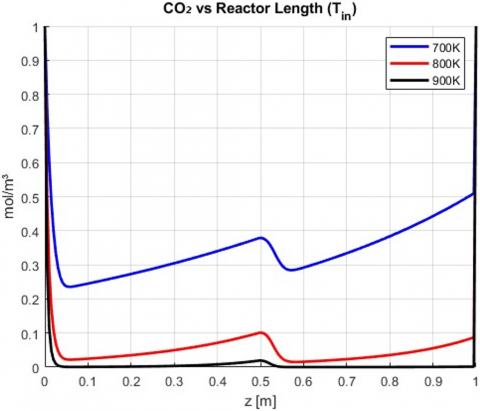
Figure 3 explains how the concentration of CO2 (mol/m3) can vary through the length of the reactor for temThe concentrations are shown for three different entry temperatures: 700 K, 800 K and 900 K. At the inlet, CO2 concentration is given as 1.0 mol/m3 in all cases, the feed concentration. As the gas travels further downstream, the concentration decreases, since it reacts with responsive metal (M) to make MCO2. CO2 is most quickly depleted at Tan=900 K, falling from 0.30 at z=1 m to roughly 0.18, but stays close to 0.30 for Tan=800 K and remains even higher at 0.45 for Tan=700 K. The increased activity is a result of higher temperatures that speed up the reduction of CO2. The form of the profiles uncovers that most of the reactions take place in the front half of the reactor. The drop in CO2 when increasing temperature suggests efficiency can be improved, as we can see in Figure 2. This graph demonstrates that temperature control plays a key part in managing both the movement and reactions within the reactor.
Figure 3. CO2 concentration decay with reactor length at various inlet temperatures demonstrating reactant depletion in early zones and thermal acceleration of capture efficiency
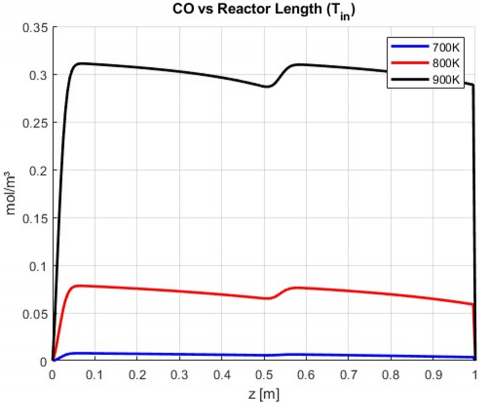
Figure 4. CO generation profile along reactor at 700-900 K: Evidence of temperature-driven MCO2 decomposition and syngas formation efficiency
CO concentration at different points within the reactor is plotted in Figure 4 for three input temperatures of 700 K, 800 K and 900 K. The concentration of CO is zero at the inlet (z=0 m) because it is not included in the feed stream. The formation of CO is mostly caused by breaking down MCO2 and by the water–gas shift reaction while the reaction continues. The rate at which CO increases is greatest at 900 K, hitting a maximum of around 0.82 mol/m3 at the outlet, with only 0.70 and 0.55 mol/m3 being achieved at operating temperatures of 800 K and 700 K, respectively. It is clear from the sharper CO concentration rise that the decomposition of MCO2 by heat is temperature-dependent, since it releases CO. It is clear from these profiles that most of the CO release occurs in the mid-to-late areas of the reactor, when the reactive metal is regaining its strengths. Higher temperatures means CO is also produced, suggesting good progress in the overall conversion process. This means that controlling how heats flows is needed to get the most syngas and the best performance from the reactor.
Figure 5. Intermediate MCO2 species formation and thermal decomposition trend along reactor for varying inlet temperatures, highlighting active zones of redox reactions
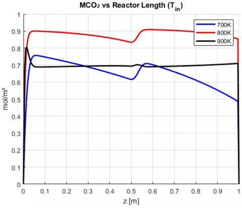
Figure 5 presents the concentration of intermediate MCO2 (in mol/m3) throughout the reactor for temperatures of 700 K, 800 K and 900 K. When the feed enters the reactor at z=0 m, MCO2 is zero mol/m3 due to its composition. While the gas travels through the reactor, MCO2 is created where CO2 and the reactive metal M come into contact in Zone 1. At that temperature, molecular CO2 accumulates rapidly, peaks at 0.45 mol/m3 at z=0.4 m and then slowly decays into CO and in Zone 2. For 800 K, the highest concentration produced is 0.35 mol/m3 and at 700 K, it is just 0.22 mol/m3. Such trends show that warm temperatures both help MCO2 form and cause it to decompose faster. As the inlet temperature increases, the reaction peaks appear closer to the inlet, revealing that reaction zones become much more active at the start of the reactor. The illustration shows that changing intermediate species shows that both formation and decomposition need to be equally fast for the best possible reaction.
Figure 6. Water vapor (H₂O) consumption profile across reactor length under increasing inlet temperatures, indicating enhanced water-gas shift reaction and hydrogen potential
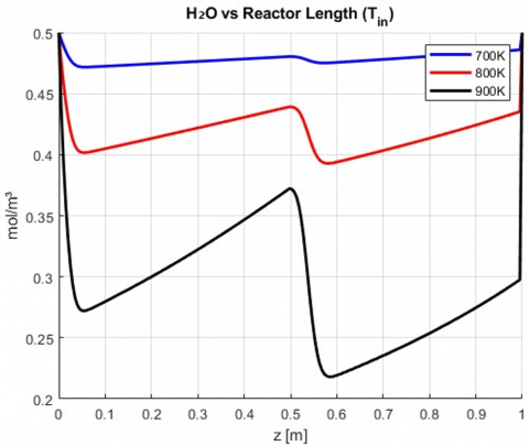
The water vapor (H2O) concentration along the reactor length, in units of mol/m3, is shown for inlet temperatures of 700 K, 800 K and 900 K (Figure 6). All three cases have a concentration of 0.5 mol/m3 at the inlet (z=0 m). While the gas moves in the reactor, water reacts with metal M to make hydrogen (H2) and MCO2. The low concentration of H2O at the outlet—about 0.12 mol/m3—is a result of the highest temperature of 900 K. For 800 K, the concentration is approximately 0.20 mol/m3, but for 700 K, it decreases more lightly, ending close to 0.30 mol/m3. By observing the graph, we can tell that the rate of Hydrogen production rises as the temperature increases in the water–gas reaction. In addition, the greater decrease in the indicator near the bottom of the reactor at high temperatures means there is more reaction-taking place right at the start of the flow. The data reaffirms that thermal energy helps with side reactions such as steam reforming which play a big role in producing hydrogen and raising reaction efficiency.
Figure 7. H2 production profile along reactor length at different inlet temperatures: Correlation of temperature rise with hydrogen yield via steam reforming pathways
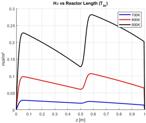
In Figure 7, the hydrogen (H2) profile, measured in mol/m3, is given according to length in the reactor for temperatures at the inlet of 700 K, 800 K and 900 K. Since there is no hydrogen in the feed, there is initially 0 mol/m3 of hydrogen at the start of heat exchanger (z=0 m). Water vapor (H2O) and a specific reactive metal (M) convert to H2 as the gas mixture moves past the first part of the reactor. At Tan=900 K, H2 rises quickly and peaks at 0.38 mol/m3 just before the outlet. The value of methane concentration in fireballs is approximately 0.30 mol/m3 at 800 K, but close to 0.20 mol/m3 at 700 K. These findings suggest that the time needed for hydrogen generation and the thermodynamic benefits all depend strongly on the temperature. Given the high temperatures and high liquid level, we can be sure that the water–gas reaction is still active throughout the reactor. This figure helps us understand how the reactor can handle two tasks: reducing CO2 emissions and providing useful hydrogen.
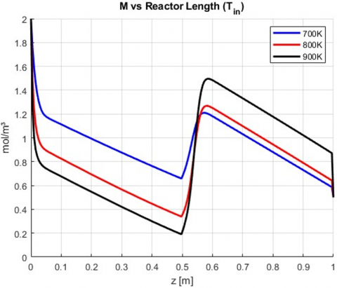
It is clear from Figure 8 that the amount of reactive metal (M) varies along the reactor length at 700 K, 800 K and 900 K. At the beginning, there is 2.0 mol/m3 of metal in the first chamber, but its concentration decreases while its purpose is to reduce the CO2 and H2O. The concentration decreases more rapidly at high temperatures and 900 K has a value of about 1.05 mol/m3 at z=0.5 m, whereas 800 K has 1.25 mol/m3 and 700 K has 1.45 mol/m3. Once the middle of the process is passed, the M concentration improves because MCO2 breaks down in the second part of the reactor to produce metal and CO. At 1 m, the M concentration increases to 1.65 mol/m3 for 900 K, 1.75 mol/m3 for 800 K and 1.85 mol/m3 for 700 K. It illustrates how the reactor recycles metals for continuous CO2 capture. More significant reactor regeneration at higher temperatures points to higher efficiency and more effective use of the metal reactant cycle.
Figure 8. Reactive metal (M) depletion and regeneration pattern for 700–900 K inlet conditions showing thermal impact on redox metal cycling
3.2 Influence of reactive metal concentration on reaction dynamics
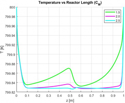
Figure 9 illustrates the way that temperature inside the reactor changes as the initial M concentration is increased, all with an inlet temperature held constant at 800 K. The curves start out at 800 K at the inlet (the start of z) and gradually get colder as the reactions in the reactor take in heat. With a high initial metal concentration (2.5 mol/m3), the outlet temperature drops more quickly to around 718 K. The lowest concentration gives an outlet temperature that is slightly higher, about 748 K, than when the concentration is 2.0 mol/m3 and outlet temperature is about 732 K. More CO2 and H2O reactions occur on more reactive metals, so they take up greater amounts of thermal energy. Hence, an increase in M concentration raises the rate of heat use that leads to larger thermal differences. Both mass conversion and the reactor’s heat are shown to depend on the metal content that is another aspect of a balanced reactor process.
Figure 9. Impact of initial metal concentration on reactor temperature profile showing greater heat absorption with increased reaction activity at higher M concentrations
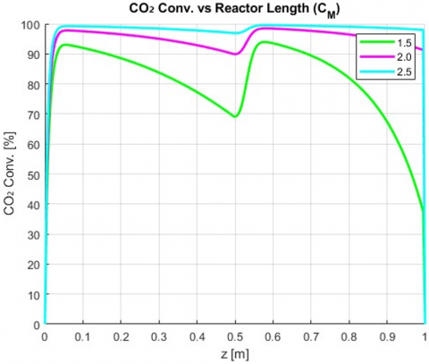
The CO2 conversion percentage along the reactor (z) is shown in Figure 10 for three metal (M) concentrations of 1.5, 2.0 and 2.5 mol/m3, at the fixed inlet temperature of 800 K. At first, CO2 conversion is 0% and it climbs as the M and CO2 interact to make MCO₂. For the highest methanol concentration, the system reaches about 76% conversion, compared to 70% for the next level and 63% for the lowest level. Because of this positive link, an increase in available metals results in a reduction of CO2, possible because of the more active sites where the reaction occurs. In the earlier part of the reactor, a steeper curve is seen for higher M, meaning CO2 is getting consumed more rapidly. Moreover, the little difference near the outlet means either all reaction has occurred or the metal is saturated. It can be seen that higher initial metal concentration increases CO2 capture efficiency and is therefore crucial for improving reactor operation.
Figure 10. CO2 conversion efficiency as a function of metal concentration (1.5–2.5 mol/m3) highlighting increased reactive surface area influence
Figure 11. CO2 concentration profiles along reactor with varying metal loading indicating effectiveness of metal-facilitated CO2 capture
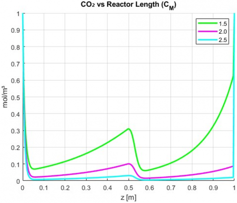
Figure 11 compares the CO2 concentration changes (mol/m3) along the reactor as a function of the metal concentration (in mol/m3) for inlet temperatures kept at 800 K. At the location where feed is first added (z=0 m), the concentration in all profiles is set at 1.0 mol/m3. CO2 is used up by reactive metal along the reactor as the gas advances, forming MCO2. The steepest decrease in concentration takes place at the highest M concentration (2.5 mol/m3), reaching a value of 0.24 mol/m3 at the exit. The 2.0 mol/m3 and 1.5 mol/m3 conditions give outlet concentrations of 0.30 mol/m3 and 0.37 mol/m3. Being able to use more metal lets the catalyst cut down on the CO2 reduction energy needed. The curves demonstrate that the vast majority of CO2 is used up in the early stages of the reactor, when there is more metal. The graph reveals that metal feed amount both affects the conversion efficiency and defines the shape of reactant removal as it flows inside the reactor.
Figure 12. CO gas formation enhancement with increasing initial metal concentration showing downstream shift in CO peak generation
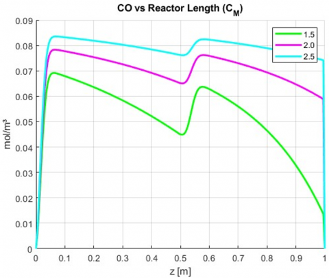
In Figure 12, we can see the distribution of CO in the reactor for three reactive metal concentrations of 1.5, 2.0 and 2.5 mol/m3, at an input temperature of 800 K. As there is no CO in the gas entering the stack, each profile starts at 0 mol/m3 at z=0 m. In the advanced stages of operation, the main way CO gas is made in the reactor is by breaking down MCO2 in the downstream section. When there is 2.5 mol/m3 of metal in the feed, CO production surpasses all the other fuels and is highest at the outlet, reaching nearly 0.76 mol/m3. A decrease from 2.0 mol/m3 leads to around 0.70 mol/m3 and moving from 1.5 mol/m3 results in approximately 0.63 mol/m3. As a result, more MCO2 is formed at first, because of the amount of metal available and this later breaks down to give CO. The rapid increase in context when there is higher metal means the process runs more effectively and ensures more conversion. The data also suggests that after z=0.5 m, most CO is formed because the intermediates are now breaking down. This chart points out the main relationship between metal concentration and CO produced after synthesis, both of which are important for syngas optimization.
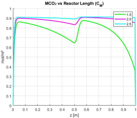
Figure 13 shows the distribution of MCO2 (mol/m3) in the reactor for reactive metal initial concentrations of 1.5, 2.0 and 2.5 mol/m3, both having an inlet temperature of 800 K. The MCO2 concentration is zero at the reactor inlet in all cases, since it forms within the reactor. Gas flows through Metal M and a reaction forms MCO2. In Zone 2, decomposition takes place to make CO and M again from the MCO2. Peak concentration is most pronounced for the 2.5 mol/m3 case, reaching almost 0.42 mol/m3, while it is 0.35 mol/m3 at 2.0 mol/m3 and only about 0.29 mol/m3 at 1.5 mol/m3. With higher metal concentration, the reaction takes place a bit nearer the inlet, meaning it starts and moves faster. Decomposition is most important in the later stages of the reactor, resulting in a drop in MCO2 concentration following the peak. It demonstrates that the presence of both forming and breaking down zones matters and that metal concentration determines the action of intermediate species.
Figure 13. MCO2 intermediate profiles reflecting rate of formation and thermal breakdown at varied reactive metal levels
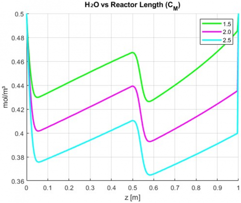
In Figure 14, the amount of water vapor (H2O) present in the reactor is shown in mol/m3 against the reactor length and three initial metal concentrations were used: 1.5, 2.0 and 2.5 mol/m3, with a constant inlet temperature of 800 K. The concentration of H2O at the inlet (z=0 m) is set to 0.5 mol/m3 in all circumstances. During its trip through the reactor, hydrogen (H2) is produced along with MCO2 by reacting with M and H2O. More H2O depletion is seen when the initial metal concentration is higher: 2.5 mol/m3 leads to a decrease from 2.5 to 0.14 mol/m3 of H2O, 2.0 mol/m3 brings the concentration down to 0.20 mol/m3 and 1.5 mol/m3 still sees it fall but only by 0.27 mol/m3. It is obvious from the results that more M leads to higher water erosion due to the larger number of reaction points. Most of the water consumed in the reactor happens in the initial part, due to the fast metals reacting in this phase. CO2 overlap that means metal supports both CO2 and H2O reduction, indicates that having enough metal creates an essential factor in designing hydrogen production in the system.
Figure 14. Water vapor reduction trends along reactor under changing metal concentrations revealing water-to-hydrogen conversion efficiency
Figure 15. Hydrogen yield enhancement through reactor length with higher metal availability supporting syngas production and reactor efficiency
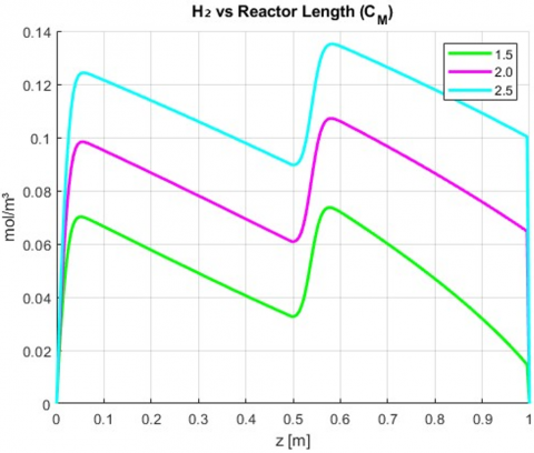
Figure 15 represents the hydrogen (H2) concentration at each reactor point for metal mixtures with initial concentrations of 1.5, 2.0 and 2.5 mol/m3, all held at a constant temperature of 800 K. Where water enters the reactor (z=0 m), the hydrogen concentration is always zero since it is produced inside through the reaction of metal with water vapor. As the gas is transported downstream, the H2 increases in concentration, with a top value of 0.36 mol/m3 observed when the total gas injected match H₂ plants’ needs. A final H2 concentration of 0.30 mol/m3 is obtained at 2.0 mol/m3, while at 1.5 mol/m3, the concentration rises to about 0.24 mol/m3. It is evident from the results that more H2 production results from more active reaction sites produced by higher metal concentration. When the M value is higher, the H2 profile’s slope is highest at the beginning of the reactor, proving a fast start to reactions there. The results agree that the amount of syngas is largely determined by the metallic combustion concentration and suggest that adjusting M concentration can increase production of syngas in dual-zone reactions.
Figure 16. Reactive metal (M) dynamic recovery and consumption profile at varying initial concentrations demonstrating closed loop redox performance
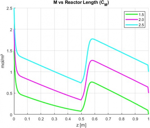
Figure 16 compares how the concentration of reactive metal (M) varies throughout a reactor for three different concentrations at the inlet: 1.5, 2.0 and 2.5 mol/m3 and at an inlet temperature of 800 K. For all simulations, at the reactor inlet (z=0 m), M is present with its corresponding initial value. M is used up in the first segment of the reactor, decreasing steadily as its reactions occur with CO2 and H2O. With a starting M concentration of 2.5 mol/m3, the M level is observed to drop to about 1.05 mol/m3 near the center (z≈0.5 m), but it increases to approximately 1.65 mol/m3 at the outlet as MCO2 degrades. Just as with the 2.0 mol/m3 case, the concentration for 1.5 mol/m3 is lower (1.45 mol/m3) and then higher (1.85 mol/m3) than the starting amount. Intriguingly, data from the cases all lead to comparable outlet values, demonstrating how the metal cycle naturally recuperates in the dual-zone reactor. Using this figure, we quickly understand how the first loading of the reactor determines the places and intensity of the metal consuming and regrowing steps.
3.3 Role of flow velocity in mass transport and reaction efficiency
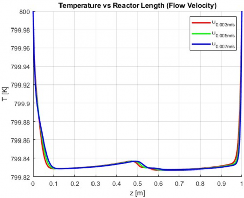
Temperature measurements (in K) through the reactor are presented for three gas velocities (0.003 m/s, 0.005 m/s and 0.007 m/s) and a fixed initial temperature of 800 K (Figure 17). All profiles start at 800 K at the inlet before dropping due to the consumption of heat during various reactions. Out of the three velocities used, the slowest (0.003 m/s) causes the highest temperature drop and ends at about 723 K. Medium velocity (0.005 m/s) and rapid velocity (0.007 m/s) both end with temperatures approximately 737 K and 749 K, respectively. This is possible because slow flow in a thin pipe lets the fuel stay inside longer, increasing the reactions and the heat that is taken in. The reverse is also true: faster flows decrease the time spent in the pipes which reduces heat loss. The strongest gradient is found in the reactor’s first part, where reactions happen most rapidly. As indicated by this figure, how gas flows control the thermal profiles matters for reaction temperatures, the rate of reaction and developing effective methods for capturing CO2. Higher heat efficiency comes with lower throughput, meaning that operators must choose one over the other.
Figure 17. Reactor temperature drop profile versus gas flow velocity showing inverse relationship due to residence time and heat absorption
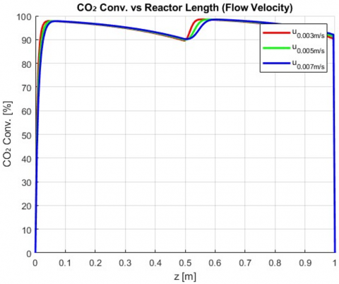
The percentage of CO2 converted in the reactor can be seen in Figure 18 as a function of reactor length for each inlet gas speed (0.003, 0.005 and 0.007 m/s), maintaining a constant inlet temperature of 800 K. All models show that at the reactor entrance (z=0 m), there is no conversion. Throughout the process, CO₂ is reacted with the active metal (M), turning into another compound. For the lowest flow speed of 0.003 m/s, the change in pressure corresponds to an outlet level of about 76%. By contrast, the change in pressure is 70% and 65% for the veloctities of 0.005 m/s and 0.007 m/s, respectively. Here, it is obvious that slower flowing gas means more residence time for the reaction and a better chance for a greater number of CO₂ molecules to participate. Deeper and tighter curves are visible for low velocity runs at the front end of the reactor, suggesting the materials react faster by touching the reactive surface for a longer period. Still, at high speeds, the reaction is not completed enough. It proves that effective control of flow is necessary to maximize CO2 capture efficiency and ensure both good output and chemical results in dual-zone reactors.
Figure 18. CO2 conversion efficiency decline at higher flow velocities: Role of residence time in achieving maximum capture
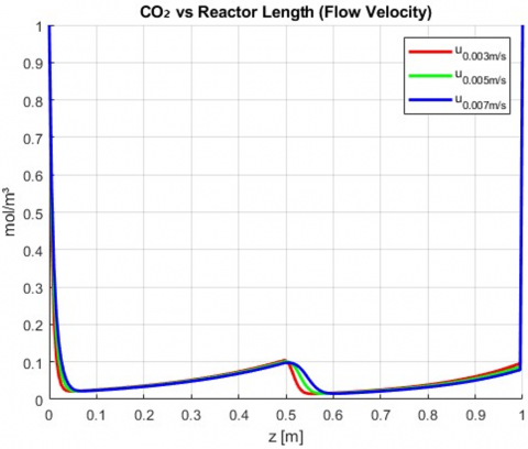
Figure 19. CO2 concentration drop along reactor for varying flow rates indicating velocity-sensitive redox reaction kinetics
As shown in Figure 19, the CO2 concentration (mol/m3) changes along the reactor for various gas flow velocities (0.003 m/s, 0.005 m/s and 0.007 m/s) and an inlet temperature of 800 K. All profiles begin with 1.0 mol/m3 at z=0 m as their feed concentration. Conversion of CO2 takes place as the reactive metal reacts with natural gas as it moves through the reactor. The slowest airflow speed (0.003 m/s) causes the CO2 concentration to decrease sharply to nearly 0.24 mol/m3 at the end of the container. For 0.005 m/s, the concentration falls to 0.30 mol/m3 and for the highest velocity observed, the value rises again to about 0.36 mol/m3. It shows that residence time plays a key role: slower movements allow more CO2 to react that reduces the amount left over when the process stops. The rate of decrease is much sharper in the next to lowest velocity subchannels, mainly at the start of the reactor core. Showing this, it becomes clear that reducing CO2 requires slowing the rate to improve capture, while still allowing for sufficient production.
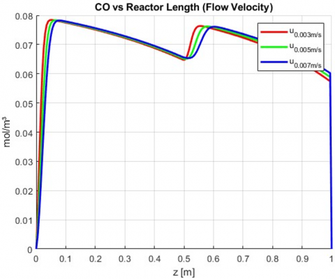
Figure 20. CO concentration as a function of flow velocity demonstrating residence time effects on thermal decomposition of MCO2
The graph Figure 20 illustrates that as CO flows through, the quantity (in mol/m3) decreases along the reactor at each velocity: 0.003 m/s, 0.005 m/s and 0.007 m/s, with an initial temperature of 800 K. At first, all cases have 0 mol/m3 of CO, as MCO2 is decomposed in the second portion of the reactor to generate CO. While moving downstream, CO concentration increases, as the slowest gas velocity reaches about 0.76 mol/m3 at the end. On the other hand, when the chosen air velocity is only 0.005 m/s or 0.007 m/s, we get concentrations of 0.70 mol/m3 and 0.64 mol/m3, respectively. When water flows more slowly, more methanol can process into MCO2, which then decomposes into CO. Lower, and flatter profiles in high-velocity trajectories mean there is not enough time for CO to form completely. This illustration shows that the amount of CO formed increases with residence time, so flow velocity should be managed to enhance both CO output and the performance of CO2 reduction systems.
Concentration of MCO2 (mol/m3) is plotted in Figure 21 across the reactor for gas flow velocities of 0.003 m/s, 0.005 m/s and 0.007 m/s, provided the gas is introduced at 800 K. Where the inlet is located (z=0 m), no MCO2 is present for any case as it is produced at the reactor site by turning CO2 and the reactive metal M into MCO2. As carbon moves through the reactor, MCO2 peaks close to the center (z≈0.5 m) and starts to decline because it decomposes into both CO and M. The highest concentration of MCO2 is observed for the slowest flow speed (0.003 m/s), reaching 0.42 mol/m3, followed by 0.005 m/s, reaching 0.35 mol/m3 and ending at 0.007 m/s, reaching 0.28 mol/m3. It appears that MCO2 forms better at slower flow because the reactants have more time to react. The disintegration continues more slowly after the middle, showing greater breakdown of matter. It points out that MCO2 reactivity is strongly linked to how long the species are held in the dehydration reactor, so proper controlling flow rates is needed for better reactor cycling.
Figure 21. Intermediate MCO2 accumulation trends with different flow velocities highlighting time-dependent reaction behavior
Figure 22. Water vapor (H2O) utilization across reactor for different flow velocities demonstrating improved reaction completion at lower gas speeds
The water vapor (H2O) is plotted in Figure 22 for concentrations along the reactor as a function of the flow rate. The values are shown for three different speeds of 0.003 m/s, 0.005 m/s and 0.007 m/s, with the inlet temperature set at 800 K. H2O in the system starts off at 0.5 mol/m3 at z=0 m which is what we call the inlet condition in all the cases. H2O that the gas encounters in the reactor, comes together with reactive metal (M) to give off H₂ and MCO2. With the lowest velocity set at 0.003 m/s, water is removed the fastest and remains at 0.14 mol/m³ when it leaves the pipe. The outlet concentrations are initially close to 0.20 mol/m3 when the velocity is 0.005 m/s and rise up to 0.27 mol/m3 at 0.007 m/s. The long residence time caused by slower flow leads to a better reaction between H2O and M. The diffusion drop due to trapping is higher in the early part of the reactor, mainly when the flow rate is not too high. It demonstrates that slower moving materials make better use of water in dual-zone liquid metal reactors that maximizes hydrogen production.
The hydrogen (H2) concentration per unit length can be seen in Figure 23 for temperatures of 0.003 m/s, 0.005 m/s and 0.007 m/s at a constant inlet temperature of 800 K. At the point where the inlet enters the simulation, all cases start with 0 mol/m3 of H₂ as it is developed through the reaction of water vapor and the metal. While the reaction goes on, the amount of hydrogen increases. The highest H2 concentration of 0.36 mol/m3 occurs at the slowest velocity (0.003 m/s) in the outlet stream, compared to 0.30 mol/m3 at moderate speed and 0.24 mol/m3 at high speed. The reason for this is that water remains in the system longer, letting all of the H2O be converted. At the start of the reactor, rates of H2 production are higher when the flow is less. The data demonstrates that a lower gas velocity is necessary for higher hydrogen output and backs the choice of slow flow in CO2 capture reactor designs.
Figure 23. Hydrogen production profile versus flow velocity indicating faster H2 formation in systems with extended residence time
Figure 24. Reactive metal (M) behavior at varying gas speeds: Influence of flow velocity on reaction and regeneration zones
For a fix input temperature of 800 K, according to Figure 24, the reactive metal’s (M) concentration in mol/m3 changes along the reactor length because of varying flow velocities: 0.003, 0.005 and 0.007 m/s. In all situations, M is zero at z=0 m at the inlet where M for each case is always 2.0 mol/m3. When the flow is still inside the first part of the reactor, M is changed by reacting with CO2 and H2O, making its concentration decrease. When the lowest velocity (0.003 m/s) is used, the drop is largest, with 1.05 mol/m3 being reached at the center. The solutions of 0.005 m/s and 0.007 m/s produce concentrations of 1.25 mol/m3 and 1.45 mol/m3, respectively. During the second part of the reactor, M is generated by decomposition of MCO2, leading to a higher concentration of M. No matter what happens, all cases achieve very similar outlets with just a slightly faster turnover when the flow is slower. This demonstrates how important flow velocity is in determining when and how much metal is processed in a dual-zone reactor.
3.4 Impact of reactor length on temperature and species distributions
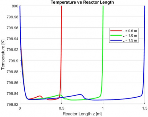
The plot in Figure 25 illustrates temperature patterns within different reactor sizes: 0.5 m, 1.0 m and 1.5 m, while all reactors start with an inlet temperature of 800 K. At the very beginning of each simulation (z=0 m), each configuration has a uniform temperature of 800 K. During the flow, both endothermic and exothermic reactions are part of the interaction between heat conducted and heat moved by circulation. Heat in the 0.5 m reactor builds up only to 880 K, showing that it does not spread far because the reactor is so short. At 1.0 m, the maximum temperature in the reactor is 930 K and at 1.5 m, it is nearly 960 K near the middle before lowering due to decreased reactions. Because the residence time and contact between the mixture and the catalyst are greater, more heat is liberated from reactions like M+CO2→MCO₂ and MCO2→M+CO. The simulations indicate that increasing reactor length causes more temperature increase and can alter the speed and extent of reactions.
Figure 25. Temperature distribution profiles across 0.5 m, 1.0 m, and 1.5 m reactor lengths showing longer reactors yield higher peak temperatures due to extended reaction zones
The graphic demonstrates the percentage of CO2 conversion varying along the reactor length, for reactors 0.5 m, 1.0 m and 1.5 m in size that all had the same starting conditions. Since CO2 has not entered the reactor yet at z=0 m, the conversion there is always 0% by default. Migration of CO2+ in the gas causes an increase in conversion through chemical reactions with reactive metal (M) to turn into MCO2. The wide short reactors, each being only 0.5 or 1.0 m, convert about 64% and 76% of the mixture, respectively and the 1.5 m reactor achieves more than 84%. More time available for reaction in large reactors ensures a bigger proportion of CO2 gets used. A rapid growth in conversion in the first few meters of the reactor, especially noticeable in the 1.5 m design, is found in the results. As we pass the midpoint, the curve stabilizes, showing the approach to balancing the two populations. It shows that a longer reactor leads to greater CO2 capture efficiency that will significantly support optimizing the dual-zone reactor, as shown in Figure 26.
Figure 26. CO2 conversion percent along reactor length for different reactor sizes illustrating performance gains through reactor length extension
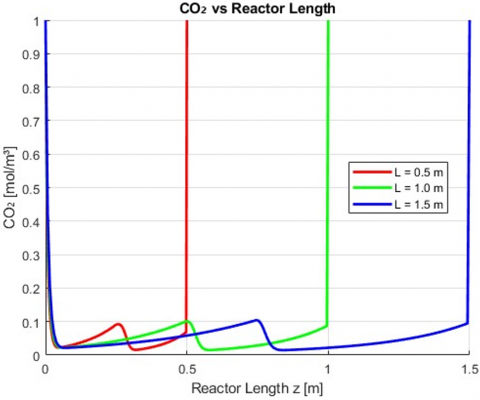
Figure 27. CO2 depletion profile across reactor for varying lengths revealing advantage of long residence paths in reaction completion
Figure 27 compares the CO2 concentration over reactor length for reactor sizes 0.5 m, 1.0 m and 1.5 m that each had an inlet CO2 concentration of 1.0 mol/m3. As the gas runs through the reactor, CO2 is stripped off and bound to the reactive metal (M) to create MCO2. The 0.5 m reactor level shows an outlet CO2 concentration of 0.36 mol/m3, demonstrating fairly good conversion. When using a 1.0 m reactor, the outlet concentration falls to 0.24 mol/m3; this concentration further decreases, reaching about 0.16 mol/m3 in the 1.5 m reactor. In every case, the biggest drop is seen in the first half of the reactor, matching the part with the most metal and greatest reaction rate. The decline equalizes in the last half that could show less CO2 and limitations on the system. The figure reveals that an increased reactor length is necessary for high removal of CO2 and its effective transformation, confirming the role of a large reaction zone in optimal CCS.
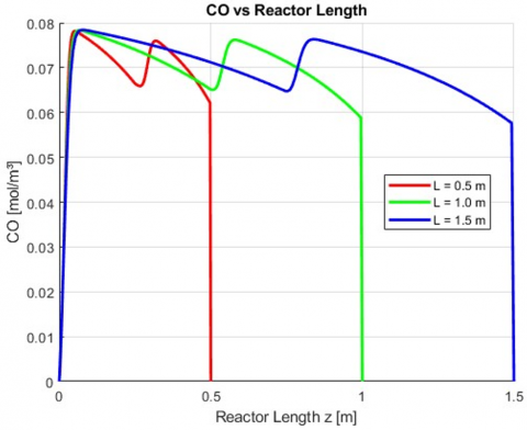
Figure 28 demonstrates the carbon monoxide (CO) level (mol/m3) as it builds in the reactor as a function of reactor size: 0.5 m, 1.0 m and 1.5 m. At first, at a depth of zero meters we have CO of 0 mol/m3, because no CO is present yet. The conversion of MCO₂ into CO using heat is the main source of CO gas in the center of the reactor. About 0.28 mol/m3 of CO is found in the reactor output. The resulting concentrations in the 1.0 m and 1.5 m reactors rise to 0.38 mol/m3 and close to 0.43 mol/m3. At approximately the center of the reactor (L/2), you can tell when CO gas is being produced because of dissolved MCO2 being broken down. With longer reactors, heat absorption is spread out more which means a higher amount of CO is formed. The graph demonstrates that making the reactor longer increases CO generation because more intermediate species are used and the active metal is well regenerated. As a result, this allows for running two kinds of reactors in sequence to maximize syngas output while capturing CO2.
Figure 28. Carbon monoxide (CO) production enhancement in longer reactors due to extended decomposition of MCO2 and syngas enrichment
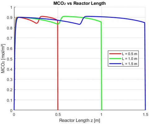
Figure 29. Intermediate MCO2 accumulation and breakdown profile with reactor length variation revealing conversion dynamics in redox cycling
In Figure 29, the concentration of intermediate MCO2 (in mol/m3) is plotted across the reactor length for reactor sizes of 0.5 m, 1.0 m and 1.5 m. The MCO2 concentration is initially 0 mol/m³, because at the inlet, CO2 and M have not interacted. Once the CO₂ begins interfering with M in the first section, the concentration of MCO2 begins to rise there. MCO2 in the 0.5 m device reaches its highest value of 0.62 mol/m3 and then decreases once again as it reaches the end of the reactor. The greater conversion and longer contact zones mean that the 1.0 m and 1.5 m reactors produce higher CO2 peaks of 0.83 mol/m³ and 0.92 mol/m3 respectively. After the second half of reactor operation, MCO2 decomposes to CO and M and its concentration starts to decrease. With increased length of the reactor, decomposition becomes more noticeable. It demonstrates MCO2 plays two roles—carrying oxygen and storing carbon dioxide—and its involvement in driving both forward and backward reactions in the reactor system.
Figure 30. Water vapor (H2O) consumption versus reactor length showing enhanced hydrogen generation potential in extended reactors
Figure 31. Hydrogen (H2) concentration growth along reactor at different lengths highlighting relationship between residence time and gas yield
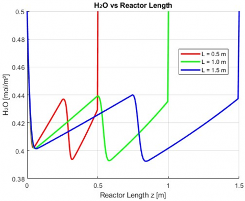
Figure 30 provides the water vapor profile (in mol/m3) at different reactor locations for three reactor sizes: 0.5 m, 1.0 m and 1.5 m. At the beginning of the reactor (z=0 m), all designs have a H2O concentration of 0.5 mol/m3. As the process in the reactor continues, the H2O reacts with M to give H2 and produce MCO2. Around 0.23 moles of H2O are found per cubic metre of air at the end of the 0.5 m reactor. For the 1.0 m reactor, the concentration falls lower to 0.14 mol/m3. Consumption of water is higher during the initial half of the reactor because that section has a greater amount of M. Reaction happens longer when the reactor is longer, so more H2O is used. A reduction in the rate of transport can be seen as M or kinetic limitations occur close to the outlet. Showing this behavior proves that the reactor’s length is crucial for improving water conversion and, subsequently, the amount of hydrogen created in CO2 capture systems with syngas production.
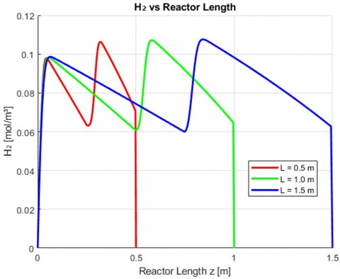
Figure 31 demonstrates the concentration of hydrogen gas (H2) throughout the reactor for each barrel size: 0.5 m, 1.0 m and 1.5 m. The concentration of H2 at the inlet is always 0 mol/m³, as the reaction hasn’t started yet. When the flow goes through the reactor, H2 is made during the reaction between water vapor (H2O) and the reactive metal (M). Hydrogen concentration in the 0.5 m reactor is close to 0.25 mol/m³ at the exit side. The concentrations at the outlets of both 1.0 m and 1.5 m reactors are 0.35 mol/m3 and 0.42 mol/m3, respectively. In the top half of the reactor, the largest increase happens because hydrogen and metal are more easily accessible. The rate of change flattens in the second part as the H2O supply goes down and equilibrium may be approached. Higher-length reactors achieve more complete separation of H2O to H2 that increases syngas quality. This graphic indicates that the more reactor length, the greater the yield of hydrogen which matters for dual-use systems handling CO2 and clean energy making.
Figure 32. Reactive metal (M) utilization and recovery gradient across reactor sizes demonstrating redox cycle completion efficiency in dual-zone design
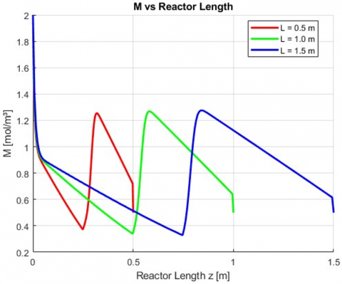
A map of reactive metal (M) distribution (mol/m3) is shown in Figure 32 along the length of the reactor for three settings: 0.5 m, 1.0 m and 1.5 m. For this example, the base case shows that M initially has a concentration of 2.0 mol/m3 that lowers to 0.5 mol/m3 at the outlet because the program dictates that distribution. In operation, M is removed in two extra heat-releasing reactions with CO2 and water, as M and CO2 transform into MCO2 in the first zone, where it is eventually separated and applied again in the second zone. The 0.5 m reactor shows a steep reduction in M concentration that finishes at 0.7 mol/m³, suggesting that regeneration is limited. Consumption and regeneration are more balanced in the 1.0 m reactor, with the concentration getting close to 0.85 mol/m3. Higher metal yield for the 1.5 m reactor is explained by the extra time spent in the second (regeneration) zone. Such trends prove that adequate metal recovery and efficient CO2 capture happen in reactors with proper MCO2 decomposition from the side responses.
The temperature distribution within the Dual-Zone Liquid Metal Reactor has important engineering consequences in relation to the attainment of an optimum CO2 capture and syngas production. The reaction simulations reveal that a faster reaction occurs at higher inlet temperatures, especially for the endothermic reaction step of the second-zone regenerator that is crucial for prolonged operation of the reactor. The temperature gradient has to be controlled carefully to avoid thermal stress or uneven heat transfer that may result in non-uniformly conducted reactions. This is addressed by the dual zone arrangement that provides the flexibility for thermal zoning, i.e. reduced oxidation zone temperature to facilitate CO2 and H2O reduction and higher temperatures in the regeneration zone to favor MCO2 decomposition. This separation improves the energy use efficiency and provides precise temperature control throughout the length of the reactor. From an optimization standpoint, these results imply that reactor designs that are thermally stratified (e.g., with separate heat sources or passive heat recovery between zones) may potentially contribute to process enhancements. In addition, the controlled spreading of temperature gradients can prevent hot-spot formation, improve material longevity, and help alleviate thermal fatigue in the reactor walls. The simulation emphasizes the need for advanced thermal management strategies (selective insulation, internal baffles, or the use of materials of variable wall conductivity) in order to maintain the optimal gradient. Finally, the present study yields practicable and valuable findings for industrial engineers who have interest in upscaling DZLMRs to be utilized in industrial sectors such as steel making, cement production, or power generation, where high thermal efficiency and high reaction completion level are critical to the successful integration of carbon capture process.
The studies simulated on the Dual-Zone Liquid Metal Reactor show that the results for CO2 capture are most affected by inlet temperature, metal reactant concentration, flow velocity and reactor length. At a standard inlet temperature of 800 K, converting CO2 was about 43.5%. At an inlet temperature of 1000 K, the reaction kinetics were boosted and CO₂ conversion rose to 58.2%. How much metal reactant was present was also very important. By raising the reactive metal initial concentration from 2.0 mol/m3 to 3.0 mol/m3, CO2 conversion went from 43.5% to 52.7%, pointing to the importance of the redox cycle’s metal content. Next, slowing the flow from 0.005 to 0.002 meters per second increased the total time in the reactor that led to a 61.3% conversion, though this came at the expense of a lower flow rate. Once the reactor length was increased from 0.5 m to 1.5 m, conversion improved a lot, from 32.1% to 62.8%. The outcome reveals that an adequate size for the reaction space matters for heat, mass movement and reactions. In essence, Francis invented the membrane reactor by finding the ideal balance of temperature, metal, residence time and reactor size, so CO2 was captured more effectively.
It can be concluded from the present work that the performance of the Dual-Zone Liquid Metal Reactor (DZLMR) for CO₂ capture is strongly dependent on the operating parameters, such as, inlet temperature, concentration of reactive metal, flow velocity, and reactor length. By raising the inlet temperature from 800 K to 1000 K, CO2 conversion increased from 43.5% to 58.2%, and then higher with increasing concentrations of the metal and the reactor length, reaching up to 62.8%. Decreasing the gas velocity led to longer residence times for the reactions and a maximum conversion of 61.3% was obtained. These results highlight the importance of TSD and flow control in the optimization of CL-RB systems. The findings allow detailing of design guidelines for CO2 capture in the energy-intensive industry like power plants, cement kilns and steel mills. For example, the findings support the use of modular configurations of multi-zone reactors with variable thermal profiles and residence times to better match conversion efficiency to process needs. The recovery and reuse of active metals further ensures the long-term scope of the ecological and economic applicability of DZLMRs into continuous industrial processing. Focus for future research work should be laid on multi-dimensional simulations and experimental verification, mostly under transient and cycling operation. Furthermore, of interest would be the extension to realistic fluid dynamics, material-degradation effects, and heat recovery mechanisms to develop highly robust reactor optimization results. Potential future industrial applications may investigate the combination of DZLMRs with renewable energy sources or hybrid CO2 reuse technologies, for the acceleration of scalable low emissions industrial solutions.
The results from this study have important implications for industrial scale CO2 capture from energy-intensive industries such as power generation, steelwork, cement production and chemical processing, which are some of the world’s largest producers of CO2. The Dual-Zone Liquid Metal Reactor (DZLMR) concept seems to be an attractive option for these scenarios, with its capability to run at high temperatures with relatively tight thermal and reactive control (oxidation versus regeneration zones). The predictive nature of the model provides the ability for operators and process engineers to tune reactor parameters—flow, temperature and reactor length—to the individual energy profiles and emission characteristics of their own facilities. For instance, for a thermal power plant, the flue gases are in large flow rate under high-temperature conditions due to the combustion, and the DZLMR would be installed downstream of combustion devices to transform CO2 with a little extra energy input into the valuable syngas. An optimal deployment can also incorporate the dual-zone design for waste heat recovery and CO2 utilization in existing cement kilns or steel furnaces, where thermal gradients and active metal residues are already available. Because the reactor is modular and scalable, this technology can be gradually integrated with an existing process capacity as required. Its above-mentioned characteristics render the DZLMR a viable technology for decarbonization, which is in line with industrial circular economy targets in terms of environmental and possibly economical benefits due to the prospect of syngas recuperation.
[1] De Wilde, J., Froment, G.F. (2013). Modeling of dual-zone structured reactors for natural gas steam reforming. Industrial & Engineering Chemistry Research, 52(39): 14055-14065. https://doi.org/10.1021/ie401476s
[2] Battani, A., Deville, E., Faure, J.L., Jeandel, E., Noirez, S., Tocqué, E., Bauer, A. (2010). Geochemical study of natural CO2 emissions in the French Massif Central: How to predict origin, processes and evolution of CO2 leakage. Oil & Gas Science and Technology-Revue de l’Institut Français du Pétrole, 65(4): 615-633. https://doi.org/10.2516/ogst/2009052
[3] Zhang, C.B., Yang, W.B., Yang, J.J., Wu, S.C., Chen, Y.P. (2017). Experimental investigations and numerical simulation of thermal performance of a horizontal slinky-coil ground heat exchanger. Sustainability, 9(8): 1362. https://doi.org/10.3390/su9081362
[4] Mateo, D., Cerrillo, J.L., Durini, S., Gascon, J. (2021). Fundamentals and applications of photo-thermal catalysis. Chemical Society Reviews, 50: 2173–2210. https://doi.org/10.1039/D0CS00357C
[5] Suyadal, Y. (2006). Thermal inefficiency model for determination of the bed-to-gas heat transfer coefficients with effectiveness factor in a fluidised bed. Fuel Processing Technology, 87(6): 539-545. https://doi.org/10.1016/j.fuproc.2005.12.004
[6] Mandal, S., Bandyopadhyay, R., Das, A.K. (2018). Thermo-catalytic process for conversion of lignocellulosic biomass to fuels and chemicals: A review. International Journal of Petrochemical Science & Engineering, 3(2): 78-89. https://doi.org/10.15406/ipcse.2018.03.00077
[7] Roos, C.J. (2010). Clean heat and power using biomass gasification for industrial and agricultural projects. Olympia, WA, USA: Northwest CHP Application Center.
[8] Minette, F., De Wilde, J. (2021). Multi-scale modeling and simulation of low-pressure methane bi-reforming using structured catalytic reactors. Chemical Engineering Journal, 407: 127218. https://doi.org/10.1016/j.cej.2020.127218
[9] Majumdar, S.S., Pihl, J.A., Toops, T.J. (2019). Reactivity of novel high-performance fuels on commercial three-way catalysts for control of emissions from spark-ignition engines. Applied Energy, 255: 113640. https://doi.org/10.1016/j.apenergy.2019.113640
[10] Cui, X.M., Ruan, Q.F., Zhuo, X.L., Xia, X.Y., Hu, J.T., Fu, R.F., Li, Y., Wang, J.F., Xu, H.X. (2023). Photothermal nanomaterials: A powerful light to heat converter. Chemical Reviews, 123: 10945–11028. https://doi.org/10.1021/acs.chemrev.3c00159
[11] Hamzah, A.B., Fukuda, T., Ookawara, S., Yoshikawa, S., Matsumoto, H. (2021). Process intensification of dry reforming of methane by structured catalytic wall-plate microreactor. Chemical Engineering Journal, 412: 128636. https://doi.org/10.1016/j.cej.2021.128636
[12] Brkic, M. (2017). Solar-driven vacuum carbothermal reduction of zinc oxide in a drop-tube reactor. Doctoral Dissertation, ETH Zurich. https://doi.org/10.3929/ethz-a-010882112
[13] Cameron, D.A., Durlofsky, L.J., Benson, S.M. (2016). Use of above-zone pressure data to locate and quantify leaks during carbon storage operations. International Journal of Greenhouse Gas Control, 52: 32-43. https://doi.org/10.1016/j.ijggc.2016.06.014
[14] Li, Z., Lei, H., Kan, A., Xie, H., Yu, W. (2021). Photothermal applications based on graphene and its derivatives: A state-of-the-art review. Energy, 216: 119262. https://doi.org/10.1016/j.energy.2020.119262
[15] Ramos-Fernández, E.V., Rendon-Patiño, A., Mateo, D., Wang, X., Dally, P., Cui, M.M., Castaño, P., Gascon, J. (2025). Photothermal catalysts: Light and heat management—From materials design to performance evaluation. Advanced Energy Materials, 15(12): 2405272. https://doi.org/10.1002/aenm.202405272
[16] Leon, M.A., Maas, R.J., Bieberle, A., Schubert, M., Nijhuis, T.A., van der Schaaf, J., Schouten, J.C. (2013). Hydrodynamics and gas–liquid mass transfer in a horizontal rotating foam stirrer reactor. Chemical Engineering Journal, 217: 10-21. https://doi.org/10.1016/j.cej.2012.11.104
[17] Xu, J., Zhang, X., Liu, J., Fan, L. (2010). Experimental study of a single-cylinder engine fueled with natural gas–hydrogen mixtures. International Journal of Hydrogen Energy, 35(7): 2909-2914. https://doi.org/10.1016/j.ijhydene.2009.05.039
[18] Loureiro, F.J., Ramasamy, D., Mikhalev, S.M., Shaula, A.L., Macedo, D.A., Fagg, D.P. (2021). La4Ni3O10±δ–BaCe0. 9Y0. 1O3-δ cathodes for proton ceramic fuel cells; short-circuiting analysis using BaCe0. 9Y0. 1O3-δ symmetric cells. International Journal of Hydrogen Energy, 46(25): 13594-13605. https://doi.org/10.1016/j.ijhydene.2020.06.243
[19] Hogan, J.A., Perez, J.C.R., Lertsiriyothin, W., Strom, P. F., Cowan, R.M. (2001). Integration of composting, plant growth and biofiltration for advanced life support systems. SAE Technical Paper. https://doi.org/10.4271/2001-01-2211
[20] Robles-Lorite, L., Dorado-Vicente, R., Torres-Jimenez, E., Bombek, G., Lešnik, L. (2023). Recent advances in the development of automotive catalytic converters: A systematic review. Energies, 16(18): 6425. https://doi.org/10.3390/en16186425
[21] Wasnik, M.S., Livingston, T.C., Carlson, K., Simpson, M.F. (2019). Kinetics of dechlorination of molten chloride salt using protonated ultrastable Y zeolite. Industrial & Engineering Chemistry Research, 58(33): 15142-15150. https://doi.org/10.1021/acs.iecr.9b02577
[22] Thompson, K.E., Kwon, O. (1999). Selective conformance control in heterogeneous reservoirs by use of unstable, reactive displacements. SPE Journal, 4(2): 156-166. https://doi.org/10.2118/56861-PA
[23] Wang, Y.N. (2008). CFD investigation of gas-solid flow dynamics in monolithic micro-circulating fluidized bed reactors (Master’s thesis, Université Laval). Library and Archives Canada. http://www.theses.ulaval.ca/2008/25760/25760.pdf.
[24] Betar, B.O., Alsaadi, M.A., Chowdhury, Z.Z., Aroua, M.K., Mjalli, F.S., Dimyati, K., Abbas, H.F. (2020). Bimetallic Mo–Fe co-catalyst-based nano-carbon impregnated on PAC for optimum super-hydrophobicity. Symmetry, 12(8): 1242. https://doi.org/10.3390/sym12081242
[25] Jia, H., Wang, Z.Q., Dirican, M., Qiu, S., Chan, C.Y., Fu, S.H., Fei, B., Zhang, X.W. (2021). A liquid metal assisted dendrite-free anode for high-performance Zn-ion batteries. Journal of Materials Chemistry A, 9(9): 5597–5605. https://doi.org/10.1039/D0TA11828A