Aminallah Rabia*![]() | Chaozhen Li
| Chaozhen Li![]() | Alessandro Biancalani
| Alessandro Biancalani![]() | Samir Yahiaoui
| Samir Yahiaoui![]() | Francisco S. Chinesta
| Francisco S. Chinesta![]()
© 2025 The authors. This article is published by IIETA and is licensed under the CC BY 4.0 license (http://creativecommons.org/licenses/by/4.0/).
OPEN ACCESS
The nonlinear dynamics of turbulence formed by the wind flowing near solid objects can be studied with a variety of different physical models, with different levels of numerical complexity. One important application is the study of the formation of turbulence past buildings, with the goal of determining the no-fly zones for drones in smart cities. In this paper, we assess the Unsteady Reynolds Averaged Navier-Stokes (URANS) model, commonly used for simulating urban wind dynamics in small portions of a city. We compare the results with those of the hybrid Large-Eddy-Simulation (URANS-LES) model, more physically comprehensive, but more numerically demanding. By analyzing the aerodynamic loads on models of drones with fixed positions close to buildings, we evaluate the implications of both models for drone flight safety. In this paper, the results demonstrate that URANS significantly underestimates these loads compared to URANS-LES approach, with discrepancies reaching a factor up to three. This highlights the need for correction strategies when relying on URANS for drone safety assessments in urban environments.
turbulence, RANS/LES, CFD, drone flight, wind, air flow over buildings
The low-altitude airspace of cities could be the streets of the future, as buildings and infrastructure will become higher rise, multifunctional and intelligent [1]. And drones could play an important role in low altitude areas as a means of transport on the streets of the future [2]. However, such environments are characterized by high population densities and complex building structures, coupled with varying weather conditions, which create unseen turbulence zones and eddies [3, 4] that have a strong negative impact on the safe travelling of drones with low inertia, slow speeds and low flight altitudes [5-7]. In order to safeguard the safe use of drones, the turbulence intensity of the zones and the impact of tangential winds on drones need to be elucidated, and based on this, no fly zones need to be set up in the city [8, 9]. The complex, nonlinear dynamics of turbulence generated by wind interacting with solid structures can be studied using various physical models, each with different levels of numerical complexity. At one end of the spectrum, Direct Numerical Simulation (DNS) resolves all turbulent scales without modeling but is prohibitively expensive for most practical urban applications. In this way Saeedi et al. [10] have performed DNS simulations for a flow over a wall mounted cylinder they find an excellent agreement with the experiment conducted by Bourgeois et al. [11] and Sattari et al. [12] in wind tunnel.
Positioned at an intermediate level of complexity, Large-Eddy Simulation (LES) and hybrid LES–RANS approaches offer a good compromise between accuracy and computational cost. These approaches resolve large-scale turbulent structures while modeling the smaller scales, allowing for improved physical realism, especially in unsteady and separated flows. This modeling strategy has been effectively applied in several studies on wind flow around buildings [13-16].
At the opposite end of the spectrum, the Unsteady Reynolds-Averaged Navier–Stokes (URANS) model is significantly more efficient computationally, as it relies entirely on time-averaged quantities to model turbulence. While this limits its ability to capture fine-scale unsteadiness and flow separation, URANS remains a practical choice for simulating large-scale urban domains. Several authors have demonstrated its capability to provide a reasonably accurate representation of the flow field while keeping computational demands manageable [17-20].
Given these considerations, one promising strategy is to combine the strengths of hybrid approaches with the efficiency of URANS by introducing suitable corrections to account for the missing dynamics.
In our previous work [21], we proposed a reduced-order model that incorporates a first-order vortex correction into the averaged wind dynamics past buildings. This approach aimed to reduce computational costs by avoiding the full expense of hybrid LES–RANS simulations while retaining essential flow features relevant for urban environments. However, that study did not explicitly quantify the implications for drone flight safety. In the present work, we extend the analysis by directly investigating the aerodynamic loads experienced by drone models positioned near buildings, comparing predictions obtained with both URANS and LES–RANS simulations. Our results demonstrate that URANS systematically underestimates the aerodynamic loads, with discrepancies reaching factor of three in highly turbulent regions, which raises concerns regarding the reliability of simplified models for operational safety. The objective of this study is therefore to provide quantitative insight into these differences and to propose improvements to the reduced model that incorporates a correction strategy based on these new findings, ultimately enhancing its relevance for defining drone safety margins in complex urban environments.
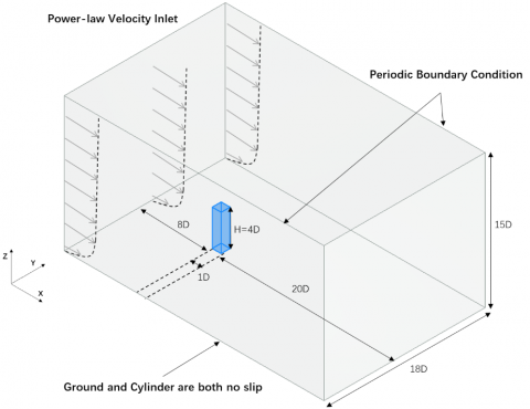
The purpose of this study is to explore the selection of turbulence models for simulating urban environments, taking the wake behind a square cylinder with aspect ratio of 4 (i.e.: $\frac{H}{D}=4$ where D is the cylinder’s width and H its height, cf. Figure 1) for Reynolds number at 12,000, as an example, to analyze the transformation of the wake and the distribution of eddies in different turbulence models, and then to add a group of small objects to simulate the load on a drone in the wake and to compare the effect experienced by the drone in the wake. The subject involves turbulence, which in this paper we resolve or model by employing two turbulence models: Delayed Detached Eddy Simulation model (DDES) [22] and $k-\omega$ Shear Stress Transport model $(k-\omega S S T)$ [23] which is a common turbulence model dealing with shedding flows. In the Delayed Detached Eddy Simulation (Hereinafter referred to as DDES) model, which is a simple modification of the nature DES model [24], a hybrid methodology is adopted, wherein the Reynolds Averaged Navier Stokes (RANS) model is applied in the near field, while the Large Eddy Simulation (LES) model is employed in the far field. This combination allows for a partial resolution of turb ulence dynamics. Consequently, the DES approach provides a more detailed representation of the flow phenomena compared to single Unsteady Reynolds Averaged Navier Stokes URANS) model.
Figure 1. Schematic of the computational domain
This paper uses the pimpleFoam solver in OpenFOAM [25] and uses the Paraview perspective for postprocessing. The second section illustrates the setup of the simulation of flow around a square cylindrical object and compares the results with publications as benchmarks, following, in the third part the simulation results of the two models DDES and $k-\omega S S T$ were compared by demonstrating the vortex structure through the Q-criterion. The fourth section combines the simulation of a square cylinder with a set of simplified models of drones to measure the load experienced by the drones in the wake. Conclusions and comments are given in the fifth section.
In this section, the predecessor information for the simulation is presented, including geometry, boundary conditions, mesh information, and governing equations.
2.1 Geometry and boundary condition
The schematic diagram of the numerical domain for the wall-mounted square cylinder (hereinafter referred to as cylinder) is shown in Figure 1.
The entire flow domain was normalized using the characteristic length scale D, defined as the width of the cylindrical obstacle. The square cylinder had a height of H=4D. The overall domain size was 29D×18D×15D, with the obstacle positioned 8D downstream of the inlet.
The Reynolds number was set to 12,000, based on the cylinder width and the freestream mean velocity. The turbulence intensity at the inlet was 0.8%. Air flowed through the domain along the x-direction, with a power-law velocity profile imposed at the inlet. A pressure boundary condition was applied at the outlet, while periodic boundary conditions were set for the front and back planes in the y-direction. The ground and square cylinder surfaces were treated as no-slip boundaries, and a symmetry condition was applied at the top of the computational domain.
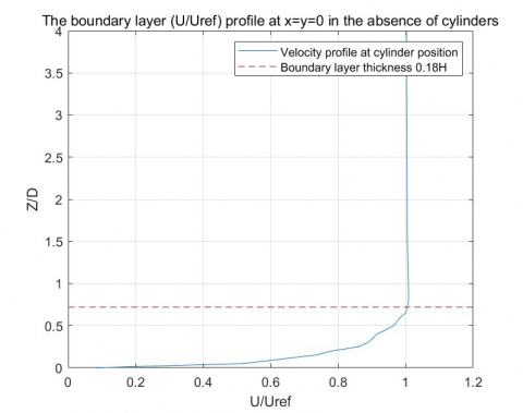
To ensure that the ground boundary layer thickness was approximately 0.18H, the inlet velocity profile was carefully prescribed. The velocity profile was measured at the obstacle’s position, as shown in Figure 2.
Figure 2. Velocity profiles boundary condition
2.2 Mesh structure
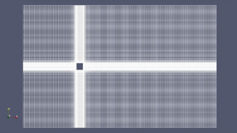
This simulation discretizes the computational domain using a structured multi-block hexahedral grid with non-uniform spacing. Local mesh refinement was implemented (stretching) in regions where significant velocity gradients were anticipated. After taking into consideration the subsequent placement of the cube within the mesh. A grid configuration of 268×208×130=7,246,720 grid cells was chosen. Within this mesh, the cylindrical region was discretized using 38×38×70 grid cells.
In this study, the mesh was designed to satisfy a target of $y^{+}<15$ where $y^{+}$ is defined as:
$y^{+}=\frac{u_\tau y}{v}$
$u_\tau$ represents the shear velocity, $y$ is the distance from the center of the cell to the nearest wall and $v$ is the kinematic viscosity.
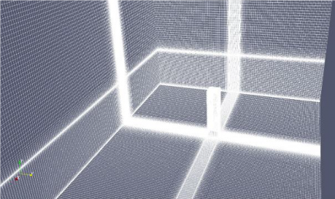
This target ensures an adequate near-wall resolution in accordance with accepted practices for DDES simulations. Although a full grid independence study was not performed due to the significant computational demand, such an analysis is identified as an important for future complementary work to further validate the robustness of the results. The 3D structure of the mesh highlighting the refined regions is shown in Figure 3 and Figure 4.
Figure 3. Schematic of the mesh structure x-y plane
Figure 4. A 3D view of the mesh structure
2.3 Simulation duration and computational time
The pimpleFoam solver employed for both simulations allow for a maximum Courant (Co) number greater than 1, with a time step of 10-4 seconds. The simulations are configured to run for a total duration of 0.5 seconds, which is equivalent to the time required for the fluid to traverse the entire computational domain 10 times. To ensure that the flow field has reached a statistically stationary state before collecting statistical data, the fluid is first allowed to flow through the entire flow field about 3 times during the simulation (the time it takes for the mean flow velocity to flow from the inlet position to the outlet plane). Comparing computational efficiency, the $k-\omega S S T$ URANS simulation, subdivided into 48 zones, necessitates approximately 35 hours for completion when executed with 48 CPU cores. In contrast, the DDES, conducted under identical conditions with the same 48 CPU cores, exhibits a slightly shorter runtime, clocking in at 30 hours.
2.4 Governing equations
In the computation of the momentum for the incompressible viscous fluid, the momentum equation is employed in this work. Each grid cell of the spatial discretization is calculated by the numerical tool OpenFOAM. The equations are expressed as:
$\frac{\partial(\rho \mathbf{V})}{\partial t}+\nabla \cdot(\rho \mathbf{V V})=\rho \mathbf{f}+\nabla \cdot \boldsymbol{\sigma}$ (1)
where, $\rho$ is the density of the fluid and $\mathbf{V}$ is the velocity vector, the $\rho \mathbf{f}$ is the volume force term and $\boldsymbol{\sigma}$ is the surface stress tensor for the cell. And the mass balance which is expressed through the continuity equation:
$\frac{\partial \rho}{\partial t}+\nabla \cdot(\rho \mathbf{V})=0$ (2)
In the case of turbulent flows a possible way is to use the so-called Reynolds decomposition by substituting (1) and (2) each unknow with the sum of an average part and a fluctuating part ($u_i=\bar{u}_i+u_{i^{\prime}}$ for velocity components and $p=\bar{p}+p^{\prime}$ for pressure) which leads to the Reynolds stresses $-\overline{u_i u_j}$.
Using the Boussinesq eddy viscosity assumption the Reynolds stresses are evaluated $-\overline{u_i u_j}=2 v_t D_{i j}$ and the eddy viscosity $v_t$ is calculated using several turbulence models. $D_{ij}$ are the components of the mean strain rate tensor. For our study we chosen a variant of the one equation Spalart-Allmaras (S-A) model [26] which intend to resolve a transport equation for the quantity $v_t$. Due to the specificity of the flow in the buffer layer and the viscous sublayer for the near-wall treattments as in our problems i.e: flow over an obstacle, S-A model uses an additional notation $\tilde{v}$ (the S-A working variable) to ensure continuity with the logarithmic layer and solve a single transport equation extending to the wall. The S-A definition for the turbulent viscosity leads to:
$v_t=\tilde{v} f_{v 1}$ (3)
$f_{v 1}=\frac{\chi^3}{\chi^3+c_{v 1}^3}$ (4)
here, $\chi=\frac{\tilde{v}}{v}, v$ is the kinematic modecular viscosity and $c_{v 1}$ is an empirical constant in the turbulence model.
$\tilde{v}$ is obtained by resolving its transport equation:
$\begin{gathered}\frac{\partial \tilde{v}}{\partial t}+u_j \frac{\partial \tilde{v}}{\partial x_j}=C_{b 1}\left(1-f_{t 2}\right) \tilde{S} \tilde{v}-\left[C_{w 1} f_w-\frac{C_{b 1}}{\kappa^2} f_{t 2}\right]\left(\frac{\tilde{v}}{d}\right)^2 \\ +\frac{1}{\sigma}\left\{\frac{\partial}{\partial x_j}\left[(v+\tilde{v}) \frac{\partial \tilde{v}}{\partial x_j}\right]+C_{b 2} \frac{\partial \tilde{v}}{\partial x_i} \frac{\partial \tilde{v}}{\partial x_i}\right\}\end{gathered}$ (5)
where, $\tilde{S}$ is the modified vorticity, $d$ is the distance to the closest wall, $\sigma$ is the turbulent Prandtl number. $C_{b 1}, C_{b 1}, C_{w 1}$ are empirical constants and $f_{v 1}, f_{t 2}, f_w$ are empirical functions of the model.
By replacing the wall-distance $d$ with a modified length scale $\tilde{d}$, which incorporates the local largest grid size $\Delta$ [24], the turbulence model becomes hybrid in nature. It behaves as the Spalart–Allmaras model when $d \ll \Delta$, and as a subgrid-scale (SGS) model when $\Delta \ll d$. This approach defines the Detached Eddy Simulation (DES) model.
The filter of the LES region is set to the third root of the volume of the cell in which it is located, the vortices with smaller scales are modeled as subgrid stresses. In contrast, the RANS model solves the mean flow field by filtering the fluctuating velocities. This also means the absence of smaller vortices in the flow field.
Finally, the DDES model is derived from the original DES formulation, with a key modification applied to the length scale that governs the eddy viscosity. This adjustment is designed to delay the transition from RANS to LES mode when the computational grid is insufficiently refined to resolve flow fluctuations. As a result, the model becomes dependent not only on the grid resolution but also on the eddy viscosity field. A comprehensive description of the DDES methodology can be found in the paper [22].
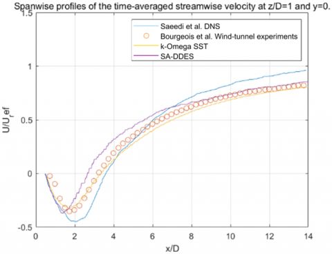
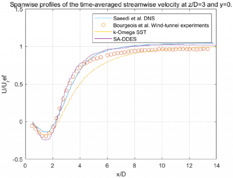
Figure 5. Benchmark of velocity profile at heights of 1/4H(top) and 3/4H(bottom)
2.5 Validation of the benchmark’s results
In this section the results of the $k-\omega S S T$ model and DDES models are presented and compared with published results to benchmark the simulations. After the 8 cycles of free stream flow through the domain, velocity data were acquired by two probe lines within the y=0 plane during $T=U r e f / D=180$ to 225. In Figures 5-7 the yellow and purple lines are from this work, benchmarked with [10, 11]. Figure 5 shows that the flow velocity is negative near the wall caused by recirculation behind the cylinder. At altitude $z=1 / 4 H$, where $x / D$ is approximately equal to 3, the value of the flow velocity is positive, but it does not return to the free-flow velocity in the range of the monitor. At higher altitudes $z=3 / 4 H$, the flow returns to free-flow velocities at a faster rate.
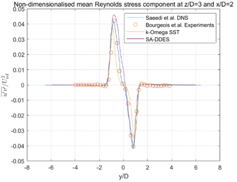
Figure 6. Benchmark of Reynolds stress component
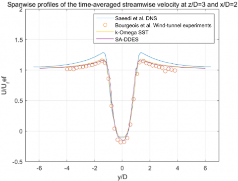
In Figure 6, the Reynolds stress curve demonstrates the most substantial negative and positive values at approximately $y / D= \pm 1$, with a steeper decline in the lateral direction. This observation implies that the shear stresses predominantly result from the interplay of vortices generated in the wake of the obstacle. As depicted in Figure 7, the time-averaged normalized streamwise velocities, taken along the lateral direction at $z / D=3$ and $x / D=2$, are presented. In the vicinity of $y / D$ ranging from -0.5→0.5, the velocity exhibits negative values, signifying the presence of recirculation within the wake. By comparison, both the $DDES$ and URANS models effectively replicate the flow patterns surrounding the cylinder.
Figure 7. Benchmark of streamwise velocity
Among the models considered, the selected DDES model closely aligns with both reference models and experimental data. Therefore, it will be used as the reference model in the following parts of our study.
In this section, the flow field around the cylinder is described and the differences between the two turbulence models are compared.
3.1 Results of DDES simulations
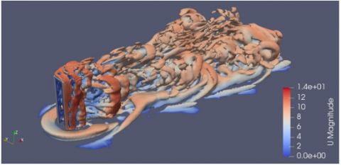
The Q criterion comes from the decomposition of the velocity gradient tensor and is employed to highlight the region of the vortex. The results in Figure 8 are from using the DDES turbulence model. These contours conspicuously reveal the detachment of the hairpin vortex structure, which is characterized by an alternating semi-annular pattern originating from the separation of the boundary layer surrounding the square cylinder. Furthermore, the shape and extent of the horseshoe vortex are clearly demonstrated on the ground ahead of the cylinder.
Figure 8. Q-criterion contours (1000) for instantaneous velocities at 0.1s in DDES colour by velocity (m/s)
3.2 Results of URANS simulations
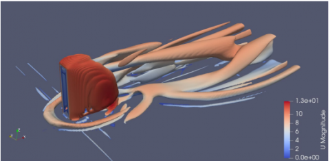
Figure 9 shows that the k-ω model effectively captures the extent and distribution of the horseshoe vortex and boundary layer. These flow features are comparable to the DDES results but do not demonstrate the shape of the hairpin vortex entrapment and capture the shedding of the boundary layer.
Figure 9. Q-criterion contours (1000) for instantaneous velocities at 0.1s in k-ω SST colour by velocity (m/s)
3.3 Comparison of URANS simulations and DDES simulations
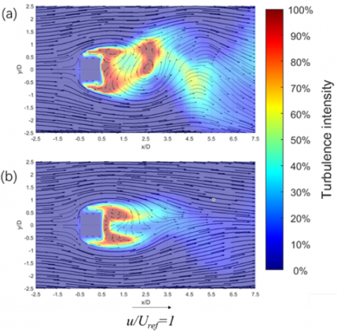
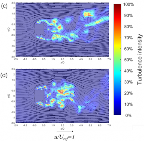
Turbulence intensity is defined as the ratio of the root mean square of the fluctuating velocity to the Reynolds mean velocity. The distribution of the turbulence intensity at different altitudes is shown in Figure 10, we could observe that in URANS the turbulence intensity is concentrated behind the cylinder, with a Karman-vortex-street like form in Figure 10(a), and in DDES the turbulence intensity is more dispersed with a higher resolution. This means that the vortices produced are on a smaller scale and are expected to be more load on small-scale drones.
Figure 10. Velocity vectors and turbulence intensity fields at 0.5s at different altitudes: (a) URANS, (b) URANS, (c) DDES at z/D=1, (d) DDES at z/D=3
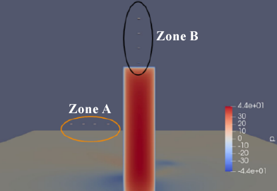
In this section, we use cubes to denote the contours of the drone to predict the forces and moments that might be experienced in the wake, with cubes of size $0.1 D \times 0.1 D \times 0.025 D$.
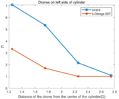
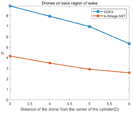
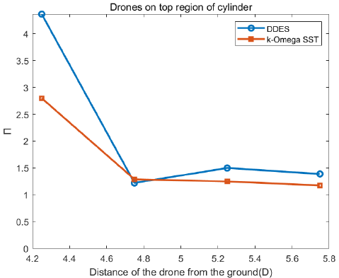
Adopt the center of the cylinder’s base as the origin, twelve drones are spatially distributed as 3 groups: (Zone A, Zone B and Zone C in Figure 11) behind the cylinder in three orthogonal directions: (1.5D, 0, 4.5D) (1.5D, 0,5D) (1.5D, 0, 5.5D) (1.5d, 0,6D) distributed in the z-direction at the back of the cylinder (Zone B), (3D, 1.25D, 2D)(3D, 1.75D, 2D)(3D, 2.25D, 2D) (3D, 2.75D, 2D) distributed in the y-direction (Zone A) and (3D, 0, 3D) (4D, 0, 3D) (5D, 0, 3D) (6D, 0, 3D) distributed in the x-direction (Zone C). Collect the maximum Cooperative effects on the drone during the simulation from time $T=U_{r e f} / D=75$ to 225, take the drone at (3D, 1.75D, 2D) from Zone A, for example. The dynamic of the cube records by forces function, it computes forces and moments by integrating pressure and viscous forces $\left(F_p, F_v\right)$ and moments in given patches. Suppose $\Pi$ is a dimensionless parameter and defined as:
$\Pi=\frac{2\left(F_p+F_v\right)}{\rho V_m^2 A}$ (6)
where, $\rho$ is the air density, $V_m$ is the average inlet air velocity and $A$ the square frontal area.
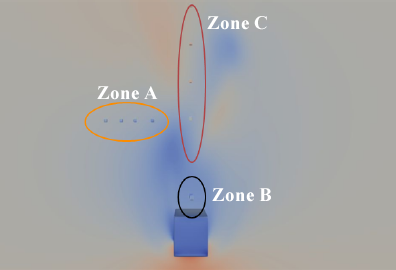
Figure 11. The location of drones: y-z plane (top), x-y plane (bottom), coloured by pressure
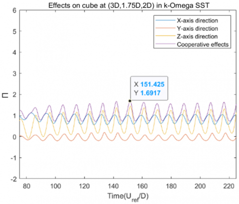
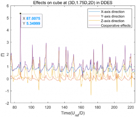
Due to the effects of shedding vortices, the force data are periodic, and the greatest contribution is the force in the z-direction. Through comparison, in DDES a sudden peak force is observed at T=87, exceedingly twice the maximum force exerted on the cube with the k-ω model, shown in Figure 12. The maximum forces acting on the three groups of drones throughout the simulation are marked and recorded. Figures 13-15 illustrate that the results of the DDES model (Blue line) exceed those in the k-ω model (red line) in the region near the cylinder, the maximum disparity between the forces encountered at the same locations can be as substantial as three times, and this difference is greater the closer the drones are to the obstacle. Both models slowly agree as the distance increases, suggesting that the DDES model is far more capable of capturing vortices in the near field than the URANS model. The group of drones situated alongside the cylinder exhibit distinct force characteristics, highlighting the disparity in the capabilities of DDES and URANS in capturing vortex interactions. The discrepancy in capturing the influence of intense eddies becomes evident in the maximum forces exerted on the cluster of drones situated behind the cylinders. In this context, DDES consistently registers forces twice as potent as URANS.
Figure 12. Force over time, k-ω (top) and DDES (bottom). Location of drone in Zone A at (3D, 1.75D, 2D)
The force acting on the drones positioned above the cylinder remains nearly identical in both models. This phenomenon is attributable to the behavior of the vortex generated by the boundary layer above the cylinder; it moves downward due to recirculation beyond the cylinder and does not expand upwards. The lowermost drone is within the boundary layer and so exhibits high forces in both models. But the slightly higher drone will be unaffected, which also demonstrates that the two models are consistent in predicting the forces on the drones in the free flow.
Figure 13. Maximum load diagram for a group of drones on the left side of the wake (Zone A)
Figure 14. Maximum load diagram for a group of drones on the back of the wake (Zone C)
Figure 15. Maximum load diagram for a group of drones on the top region of the wake (Zone B)
Based on the results obtained and considering that the aerodynamic loads predicted by URANS can be underestimated by up to a factor of two compared to DDES, we define the critical region requiring correction as bounded from the center of the cylinder by x < 6D in the downstream, y < ±2D on the side, and z < 4D at the top of the cylinder. We therefore recommend performing an initial URANS simulation, followed by applying a correction factor of two to the loads estimated on drone models within this specified region. Once corrected, the resulting load levels should be compared to the safety thresholds specific to each drone, acknowledging that drone stability and safety characteristics may vary depending on the technology and manufacturer specifications. Finally, by comparing the safety margins proposed in our previous study [21] with those obtained here, a more informed decision can be made regarding whether the no-fly zones can be reduced while maintaining operational safety. It is important to emphasize that this study is to evaluate the aerodynamic loads experienced by a drone positioned at specific locations within the turbulent wake of buildings, in order to assess whether the drone's design and stabilization technologies are sufficient to operate safely in such conditions. The detailed analysis of dynamic responses, such as attitude changes or control system reactions, is beyond the scope of this work but represents an interesting direction for future research.
In this work, the wake behind a square cylinder for Reynolds number Re=12000 is studied. The wind is modeled using different turbulence models: Delayed Detached Eddy Simulation and k- Omega Shear Stress Transport model. The load measured for a group of drones (simplified as a cube) placed at different locations in the turbulent wake. It can give insights into later studies of forces on drones in turbulence or studies of turbulence distribution in cities. In Section 3, we visualize the turbulence in both simulations using the Q-criterion, compared to URANS, in DDES the vortices are smaller and more widely and farther spread out. The important difference between these two results is the size of the vortices they produce: the size of the vortices in the DDES is comparable to the size of the drone, whereas the URANS model produces vortices on a much larger scale than the drone, despite the fact that the two models have comparable mean velocity profiles and Reynolds stress distributions. In Section 4, we compare the different turbulence models by placing cubes at different locations to simulate aerodynamic forces on drones. Notably, DDES excels in accurately capturing the risk associated with force fluctuations, thanks to its careful treatment of intricate turbulence. In contrast, the RANS model underestimates drone forces close to the cylinder, by a factor of three at some locations, it also underestimates the extent of the turbulence distribution. Where the DDES model predicts no turbulence distribution, such as the region above the cylinder, the two models’ results were comparable. We can conclude that when the turbulent structures are at the same scale as the drone, the drone is subjected to greater loads. Given the URANS model’s cost advantage and the great grid demands in urban simulations, it is still a practical choice. However, by comparing the two models, we have revealed some shortcomings of the URANS model. As a practical recommendation, the findings suggest that within the critical near-wake region identified around buildings, aerodynamic loads predicted by URANS simulations should be corrected by an appropriate factor estimated here up to two to better reflect the more realistic loads captured by higher-fidelity models. This correction can improve the reliability of safety assessments for drones operating in complex urban environments, while also providing a computationally efficient alternative to full hybrid simulations.
Building on the findings of this study, several perspectives can be considered to reinforce and expand the current work. While our numerical results highlight significant discrepancies in the estimated aerodynamic loads on drones exposed to urban turbulence, experimental validation remains essential. Prior studies by Abdulrahim et al. [5] and Paz et al. [9] have shown that low-inertia drones are highly sensitive to vortex structures generated near buildings, reinforcing the need to compare simulations results with wind tunnel experiments or real-flight measurements using onboard sensors or telemetry systems. In addition, integrating the turbulence zone predictions with existing regulatory resources such as the FAA’s UAS Facility Maps [27] or the French DGAC’s portal "Géoportail Drones" [28] would provide a practical means to assess how aerodynamic constraints intersect with currently flight restrictions. This approach could support the definition of refined safety margins or suggest the preferential flight corridors based on quantitative aerodynamic criteria. Moreover, inspired by the work of Gao et al. [8], the incorporation of local meteorological data, including wind intensity and turbulence levels, represents a key step toward the development of operational tools for real-time trajectory planning in complex urban environments. These observations collectively suggest that future modeling efforts should place greater emphasis on trajectory planning and avoidance strategies, rather than focusing solely on model accuracy within such complex flow regions. Additionally, it is essential to recognize that the actual dynamic response of a drone in real-world conditions may differ significantly from numerical predictions. As such, the validation of simulation models against experimental or in-flight data remains an important challenge for future research.
Alternatively, Reduced-Order Models (ROM) can be used to simplify the complexity in urban simulations by retaining key features and using techniques such as Proper Orthogonal Decomposition (POD) or Principal Component Analysis (PCA) to construct ROMs to achieve a model that can be used in urban simulations using DDES in subsequent studies.
[1] Stenvot, L. (2021). Leading CNRS project on hybrid AI launched in Singapore. https://news.cnrs.fr/articles/leading-cnrs-project-on-hybrid-ai-launched-in-singapore.
[2] Mohsan, S.A.H., Khan, M.A., Noor, F., Ullah, I., Alsharif, M.H. (2022). Towards the unmanned aerial vehicles (UAVs): A comprehensive review. Drones, 6(6): 147. https://doi.org/10.3390/drones6060147
[3] Letzel, M., Helmke, C., Ng, E., An, X., Lai, A., Raasch, S. (2012). LES case study on pedestrian level ventilation in two neighbourhoods in Hong Kong. Meteorologische Zeitschrift, 21(6): 575-589. https://doi.org/10.1127/0941-2948/2012/0356
[4] Blocken, B., Stathopoulos, T., van Beeck, J.P.A.J. (2016). Pedestrian-level wind conditions around buildings: Review of wind-tunnel and CFD techniques and their accuracy for wind comfort assessment. Building and Environment, 100: 50-81. https://doi.org/10.1016/j.buildenv.2016.02.004
[5] Abdulrahim, M., Watkins, S., Segal, R., Marino, M., Sheridan, J. (2010). Dynamic sensitivity to atmospheric turbulence of unmanned air vehicles with varying configuration. Journal of Aircraft, 47(6): 1873-1883. https://doi.org/10.2514/1.46860
[6] Lissaman, P. (2009). Effects of turbulence on bank upsets of small flight vehicles. In 47th AIAA Aerospace Sciences Meeting Including the New Horizons Forum and Aerospace Exposition, Orlando, Florida. https://arc.aiaa.org/doi/abs/10.2514/6.2009-65
[7] Pisano, W., Lawrence, D. (2009). Control limitations of small unmanned aerial vehicles in turbulent environments. In AIAA Guidance, Navigation, and Control Conference, Chicago, Illinois. http://doi.org/10.2514/6.2009-5909
[8] Gao, M., Hugenholtz, C.H., Fox, T.A., Kucharczyk, M., Barchyn, T.E., Nesbit, P.R. (2021). Weather constraints on global drone flyability. Scientific Reports, 11: 12092. https://doi.org/10.1038/s41598-021-91325-w
[9] Paz, C., Suárez, E., Gil, C., Baker, C. (2020). CFD analysis of the aerodynamic effects on the stability of the flight of a quadcopter UAV in the proximity of walls and ground. Journal of Wind Engineering and Industrial Aerodynamics, 206: 104378. https://doi.org/10.1016/j.jweia.2020.104378
[10] Saeedi, M., LePoudre, P.P., Wang, B.C. (2014). Direct numerical simulation of turbulent wake behind a surface-mounted square cylinder. Journal of Fluids and Structures, 51: 20-39. http://doi.org/10.1016/j.jfluidstructs.2014.06.021
[11] Bourgeois, J., Sattari, P., Martinuzzi, R. (2011). Alternating half-loop shedding in the turbulent wake of a finite surfacemounted square cylinder with a thin boundary layer. Physics of Fluids, 23: 095101. https://doi.org/10.1063/1.3623463
[12] Sattari, P., Bourgeois, J.A., Martinuzzi, R.J. (2012). On the vortex dynamics in the wake of a finite surface-mounted square cylinder. Experiments in Fluids, 52: 1149-1167. https://doi.org/10.1007/s00348-011-1244-6
[13] Paterson, D.A., Apelt, C.J. (1990). Simulation of flow past a cube in a turbulent boundary layer. Journal of Wind Engineering and Industrial Aerodynamics, 35: 149-176. https://doi.org/10.1016/0167-6105(90)90214-W
[14] Yousif, M.Z., Lim, H.C. (2021). Improved delayed detached-eddy simulation and proper orthogonal decomposition analysis of turbulent wake behind a wall-mounted square cylinder. AIP Advances, 11: 045011. https://doi.org/10.1063/5.0045921
[15] Chang, C.H., Meroney, R.N. (2001). Numerical and physical modeling of bluff body flow and dispersion in urban street canyons. Journal of Wind Engineering and Industrial Aerodynamics, 89(14-15): 1325-1334. https://doi.org/10.1016/S0167-6105(01)00129-5
[16] Zedan, A.S.A., Ayad, S.S., Abdel-Hadi, E.A., Gaheen, O.A.M. (2006). Large eddy simulation for flow around buildings. In Proceedings of ICFDP 8: Eighth International Congress of Fluid Dynamics and Propulsion, Sharm El-Shiekh, Egypt.
[17] Gorlé, C., van Beeck, J., Rambaud, P. (2010). Dispersion in the wake of a rectangular building: validation of two Reynolds-averaged Navier–stokes modelling approaches. Boundary-Layer Meteorology, 137: 115-133. https://doi.org/10.1007/s10546-010-9521-0
[18] Balogh, M., Parente, A., Benocci, C. (2012). RANS simulation of ABL flow over complex terrains applying an Enhanced k-ε model and wall function formulation: Implementation and comparison for Fluent and OpenFOAM. Journal of Wind Engineering and Industrial Aerodynamics, 104-106: 360-368. https://doi.org/10.1016/j.jweia.2012.02.023
[19] Longo, R., Ferrarotti, M., Garcı́a Sánchez, C., Derudi, M., Parente, A. (2017). Advanced turbulence models and boundary conditions for flows around different configurations of ground-mounted buildings. Journal of Wind Engineering and Industrial Aerodynamics, 167: 160-182. https://doi.org/10.1016/j.jweia.2017.04.015
[20] Richards, P.J., Hoxey, R.P. (1993). Appropriate boundary conditions for computational wind engineering models using the k-∈ turbulence model. Journal of Wind Engineering and Industrial Aerodynamics, 46-47: 145-153. https://doi.org/10.1016/0167-6105(93)90124-7
[21] Maiti, S., Rabia, A., Ammar, A., Biancalani, A., Chinesta, F., Hoarau, Y., Yahiaoui, S. (2024). A reduced model retaining 1st-order vortex corrections in the averaged dynamics of the wind past buildings. International Journal of Heat and Technology, 42(5): 1534-1540. https://doi.org/10.18280/ijht.420506
[22] Spalart, P.R., Deck, S., Shur, M.L., Strelets, M.K., Travin, A., Squires, K.D. (2006). A new version of detached-eddy simulation, resistant to ambiguous grid densities. Theoretical and Computational Fluid Dynamics, 20: 181-195. https://doi.org/10.1007/s00162-006-0015-0
[23] Menter, F.R. (1994). Two-equation eddy-viscosity turbulence models for engineering applications. AIAA Journal, 32(8). https://doi.org/10.2514/3.12149
[24] Spalart, P.R., Jou, W.H., Strelets, M., Allmaras, S.R. (1997). Comments on the feasibility of LES for wings, and on a hybrid RANS/LES approach. In Proceedings of the First AFOSR International Conference on DNS/LES, Ruston.
[25] Foundation, OpenFoam, OpenFOAM: The Open Source CFD Toolbox, https://openfoam.org, 2023.
[26] Spalart, P.R., Allmaras, S.R. (1994). A one-equation turbulence model for aerodynamic flows. In 30th Aerospace Sciences Meeting and Exhibit, Reno, U.S.A., pp. 5-21. https://doi.org/10.2514/6.1992-439
[27] Federal Aviation Administration (FAA), UAS facility maps. https://faa.maps.arcgis.com.
[28] Direction Générale de l'Aviation Civile (DGAC), Géoportail Drones. https://www.geoportail.gouv.fr/donnees/restrictions-usage-drones-loisir.