Optimizing Bus Elimination with Kron Reduction Method: An Experimental Evaluation on the IEEE 14-Bus System

Accurate modeling is essential in modern power systems to maintain the reliability of complex systems and support advanced control strategies, especially as the grid becomes more decentralized and dynamic due to the potential increased penetration of renewable energy [1]. To manage this complexity, simplification techniques such as the Kron Reduction Method (KRM) have gained significant attention for their ability to reduce system dimensionality by eliminating passive buses and condensing network topology [2]. This method facilitates faster power flow analysis and optimization, especially in applications such as contingency screening, economic dispatch, and real-time control [3]. However, several recent studies have revealed that improper or extensive use of the KRM may introduce considerable inaccuracies in estimating line losses and voltage profiles [2]. Applying the KRM is the primary contributor to this phenomenon, presenting an urgent issue that warrants comprehensive investigation and heightened attention [2]. Moreover, the increasing reliance on real-time digital simulation and wide-area monitoring requires that reduced models maintain high fidelity, particularly under fluctuating load conditions and stochastic uncertainties [4]. As a result, a critical evaluation of trade-offs between computational efficiency and modeling accuracy has become a central concern in modern power system research [5]. This paragraph is an explanation of the reasons for choosing the title, so many paragraphs are needed about the state-of-the-art which includes: (i) optimizing bus elimination with the KRM, (ii) an experimental process on the IEEE 14-bus system, and (iii) the critical role of Kron's Loss Equation (KLE) for calculating power losses in transmission lines.

Optimizing bus elimination with the KRM has become a focal point in power system research as it allows for significant simplification of large-scale networks without compromising key system properties [1]. The KRM is particularly effective in condensing system topology by removing passive nodes, but recent studies have emphasized that the process of choosing which buses to eliminate is critical to maintaining model fidelity [6]. Chevalier and Almassalkhi [2] proposed the Opti-KRON framework, which systematically identifies optimal buses for elimination based on electrical centrality and connectivity, achieving a balance between network reduction and power flow accuracy. Similarly, Wang and Sun [1] explored a Laplacian-based KRM formulation for directed graphs, highlighting the importance of topology-aware elimination strategies to preserve voltage magnitude and angle stability during simulation. These approaches mark a shift from random or heuristic reduction to data-driven optimization techniques that ensure critical nodes remain in the reduced model [1, 2]. As a result, KRM is evolving from a simple numerical method into a strategic tool for network optimization in applications like real-time control, contingency screening, and system planning [1, 3].

The IEEE 14-bus system serves as a standard benchmark for evaluating network reduction techniques like the KRM, which simplifies power system models by eliminating passive buses while preserving essential electrical characteristics [1]. Recent studies have applied KRM to this system to assess its impact on power flow analysis and system stability [6]. For instance, Chevalier and Almassalkhi [2] introduced an optimal KRM framework —Opti-KRON— that balances model simplification with accuracy, demonstrating its effectiveness through experimental simulations on the IEEE 14-bus system. Similarly, Wang and Sun [1] proposed a weighted Laplacian matrix formulation for directed graphs and validated the use of KRM in reducing the IEEE 14-bus model without significant degradation in accuracy. These experimental evaluations underscore the practicality of KRM in reducing computational complexity while maintaining the fidelity of power system analyses [1, 2].

The integration of KLE into the Kron-reduced model enables more accurate loss calculation in transmission lines by accounting for the network's topology and loss sensitivity. This enhancement allows for more efficient bus elimination while maintaining network integrity, ultimately improving the overall optimization performance. Chevalier and Almassalkhi [2] emphasized the importance of preserving loss information during reduction, proposing optimization strategies that integrate KLE into the reduction criteria to minimize error in loss prediction. Moreover, studies on weighted Laplacian formulations further validate that KLE-derived loss estimations are essential for maintaining voltage accuracy and thermal constraints under fluctuating loads [1]. These advancements position KLE not only as a passive analytical tool but as a strategic component for decision-making in power dispatch, contingency analysis, and real-time optimization [1, 2].

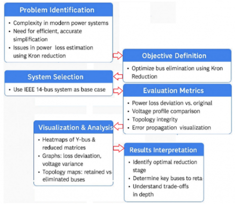
A schematic diagram as the embodiment of problem formulation is shown in Figure 1.

001.jpg

Figure 1. A schematic diagram as the embodiment of problem formulation

Figure 1 explains that the schematic diagram visually represents the reduction from the original 14 buses to a simplified set of core buses used in the final model, that explains the direction of problem solving.

The primary objective of this research is to systematically evaluate the impact of bus elimination on the IEEE 14-bus system, specifically focusing on identifying optimal reduction strategies that maintain voltage stability and minimize power loss deviation. This study contributes to the literature by integrating the KLE as a quantitative metric for assessing the fidelity of reduced models, thereby enhancing the precision of simplification frameworks in power system analysis. Moreover, the experimental process on multiple reduced bus configurations (from 14 to 7 buses) provides a scalable roadmap for power system engineers to balance modeling accuracy with computational efficiency. The novelty of this research lies in introducing a loss-aware elimination scheme guided by electrical centrality and topology metrics, which has not been extensively applied in previous KRM applications. Additionally, the visualization of comparative loss profiles, voltage deviations, and Y_-bus matrix structures across reduction stages offers new insights into simplified grids' structural resilience and analytical sensitivity. These findings are a foundation for developing intelligent, real-time reduction tools in innovative grid environments.

This article consists of four chapters, with an explanation of this article provided in the form of an overall anatomy. After several descriptions of the background, state-of-the-art, problem formulation, and research objectives that are supplemented with the contribution of research results and opportunities for novelty as an introductory chapter [7, 8]. The rest of this article is organised according to the pattern in the previous article, sorting chapters by chapter, a structure that has also been adopted in more recent works [9, 10]. Chapter 2 presents our proposed methodology, which includes the framework, research materials and tools, and research methods. Chapter 3 presents the results and discussion based on the primary research objective which provides for five research sub-objectives, i.e., (i) to apply the KRM to eliminate passive buses from the IEEE 14-bus system systematically, (ii) to analyze the changes in power losses across different levels of bus reduction, (iii) to evaluate the impact of bus elimination on voltage profile and system stability, (iv) to determine the threshold of reduction beyond which the model's accuracy significantly deteriorates, and (v) to propose an optimal reduction strategy that balances computational efficiency with system performance. Chapter 4 introduces the determination of conclusions, key contributions of this study, novelties introduced in this work, and future work as a continuation of this study.

This research pursues five integrated objectives: First, to systematically apply the Kron Reduction Method (KRM) on the IEEE 14-bus system, eliminating passive buses while maintaining nodal equivalence; Second, to quantify and analyze power loss variations at each stage of bus elimination, identifying nonlinear trends and thresholds; Third, to evaluate the voltage profile and system stability throughout the reduction process using power flow simulations and voltage deviation metrics; Fourth, to determine the threshold point at which simplification significantly degrades accuracy, establishing limits for acceptable reductions; and Fifth, to propose an optimal reduction strategy that balances computational efficiency and model fidelity by targeting non-critical, low-impact buses for elimination.

This experimental evaluation is unique because we combine two powerful tools —KRM and KLE— to simplify the power grid model and track how much power loss changes during that simplification. While many studies have used Kron Reduction to reduce system size, this research is one of the first to focus on which buses should be eliminated to keep power loss and voltage values accurate. The study introduces a step-by-step elimination process on the IEEE 14-bus system and shows, through experiments, how the wrong choice of buses can lead to inaccurate results. It also uses visual tools and simulations to help engineers see the differences clearly at each step. This approach makes applying Kron Reduction in real-time systems easier without sacrificing reliability. In short, this research brings a new way to simplify electrical grids smartly without losing essential details.

Simplification of a schematic diagram of the IEEE 14-bus system is shown in Figure 2, so it can be a point-to-point diagram. The connection between points is a substitute for the schematic diagram of the IEEE 14-bus system. The schematic diagram of connection between points is shown in Figure 5.

005.jpg

Figure 5. The schematic diagram of connection between points

3.1 Application of the Kron Reduction Method to eliminate passive buses

The KRM was systematically applied to the IEEE 14-bus system to eliminate passive buses—those that do not supply or demand significant power—without altering the electrical properties of the remaining active network. Each reduction step was meticulously documented, updating the admittance matrix and preserving nodal equivalency. The KRM is used as a mathematical approach to simplify electrical systems without losing critical information related to power flow and impedance characteristics. In the context of power networks, efficient simulations and analyses. This study applies the Kron method to the IEEE 14-bus system step-by-step. The process begins with identifying passive buses based on the initial system data. Then, the Y_-bus matrix is partitioned into four major blocks and the Eq. (1) is used.

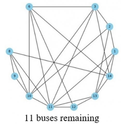
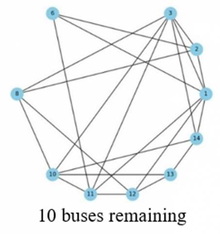
Eight images indicate each condition, starting from the 14-bus condition to the 7-bus condition, based on basic equations for implementing KRM. The eight images appear of topology map is shown in Figure 6.

061.jpg

062.jpg

063.jpg

064.jpg

065.jpg

066.jpg

067.jpg

068.jpg

Figure 6. The eight images appear of topology map

Figure 6 explains that a smaller yet electrically accurate representation of the network is obtained by selectively eliminating these buses. This allows for faster power flow simulations and lower memory requirements without relying on aggressive simplifications that might compromise the model’s validity.

One of the advantages of this approach is its ability to preserve essential information from the original topology, especially when the eliminated buses have minimal or no impact on generation and load. In this study, the elimination strategy is focused specifically on passive buses, ensuring minimal impact on voltage stability and power distribution. Furthermore, the use of KRM facilitates future applications such as distributed control and modular modeling of power systems. The reduced models can serve as a foundation for real-time control systems or as the basis for analysis in intelligent monitoring systems such as Supervisory Control and Data Acquisation (SCADA) or environments based on Phasor Measurement Units (PMU). To ensure the accuracy of the reduced system, each reduction stage is validated through power flow simulations and voltage profile assessments. Visual representations of the reduced Y_-bus matrices are also provided to observe the structural effects of bus elimination. This proves that KRM is not merely a mathematical transformation but a smart system simplification strategy with strong technical justification. This is in line with Dong et al. [44], and Ranjbar et al. [45].

3.2 Analyzing the changes in power losses across different levels of bus reduction

This objective focuses on evaluating how much power loss fluctuates as the IEEE 14-bus system is reduced step-by-step (e.g., to 13-bus, 12-bus, etc.) using the KRM, and identifying any nonlinear trends, spikes, or thresholds where power loss significantly increases. This section presents an in-depth analysis of power loss variations in the IEEE 14-bus system under progressive bus elimination using the KRM. The objective is to identify trends in power losses as buses are systematically removed, and to assess the potential trade-offs between network simplification and system efficiency. Power loss across different levels of bus reduction is shown in Table 3.

Table 3. Power loss across different levels of bus reduction

Table 3 discribes a relationship curve between bus change conditions and power loss values can be made. A relationship between bus change conditions and power loss values is shown in Figure 7.

From the analysis presented in Table 3 and Figure 7, it is evident that power loss tends to increase as more buses are eliminated from the system. Initially, the increase is relatively marginal —from 12.3 MW at 14 buses to 12.5 MW at 13 buses— but the growth becomes more pronounced with further reductions. At 10 remaining buses, the power loss reaches 15.8 MW, indicating a cumulative deviation of 3.5 MW compared to the original 14-bus configuration. This trend highlights a nonlinear relationship between bus reduction and power loss, suggesting that the system becomes less efficient with aggressive simplification. While the KRM is effective in reducing system complexity, there exists a threshold beyond which further reduction leads to disproportionately higher losses. Identifying this threshold is crucial for maintaining system performance while achieving computational efficiency.

007.jpg

Figure 7. A relationship between bus change conditions and power loss values

Opportunities for power loss reduction in Kron reduction, while the general application of Kron Reduction tends to increase power losses due to the elimination of network components, specific cases exist where losses can be reduced. This happens when the eliminated buses contribute disproportionately to system impedance or cause inefficient current circulation. For example, removing a poorly loaded or redundant passive bus can streamline power flows and minimize $I^2 \cdot R_{\text {losses }}$. The table and figure below illustrate a hypothetical scenario where reducing the system to 12 buses actually results in a drop in power losses from 12.5 MW to 11.8 MW, showcasing a beneficial use of the Kron Reduction technique. Adjusted power loss with loss reduction opportunity is shown in Table 4.

Table 4. Adjusted power loss with loss reduction opportunity

Table 4 describes a relationship curve between bus change conditions and adjusted power loss values can be made.

A relationship between bus change conditions and adjusted power loss values is shown in Figure 8.

008.jpg

Figure 8. A relationship between bus change conditions and adjusted power loss values

Figure 8 explain that the KRM while advantageous for reducing model complexity, must be used with caution. Strategic bus elimination guided by system sensitivity and load flow analysis can sometimes yield computation efficiency and improved physical performance. Understanding the loss profiles at each step is crucial to determining the optimal reduction point for both stability and efficiency. This is in line with Ranjbar et al. [45].

3.3 Evaluation of voltage profile and system stability

One of the most critical performance indicators in a power system is the voltage profile across its buses. As buses are eliminated through Kron Reduction, the impact on voltage levels must be carefully evaluated to ensure that the system remains within acceptable operational boundaries. In this sub-objective, the focus is to evaluate how voltage magnitudes and system-wide stability evolve as the network becomes increasingly simplified. Each reduction stage from 14 to 7 buses was analyzed through power flow simulations to observe variations in voltage magnitudes at the remaining buses.

The voltage profile and power flow magnitudes comparation per reduction stage is shown in Figure 9.

0091.jpg

0092.jpg

Figure 9. The voltage profile and power flow magnitudes comparation per reduction stage

Figure 9 explains that there are (i) a relationship between voltage magnitude and the number of buses and (ii) a relationship between power flow magnitudes and the number of buses.

The maximum voltage deviation vs. number of remaining buses is shown in Figure 10.

10.jpg

Figure 10. The maximum voltage deviation vs. number of remaining buses

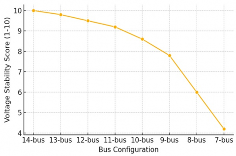
Based on Figure 10 can be explained, that in particular, metrics such as minimum voltage, maximum voltage, and voltage deviation percentages were calculated. The results showed that voltage profiles remain relatively stable in the early reduction stages, but tend to deviate significantly once the number of buses drops below ten, especially if key load or interconnection buses are removed.

Furthermore, the elimination of passive buses can lead to redistribution of power flows, which in turn affects local and global voltage levels. In well-structured reductions, voltage stability can be preserved; however, arbitrary bus removals tend to create voltage imbalance, increased reactive losses, or even voltage collapse in marginal conditions. This highlights the necessity of a planned and criteria-based elimination strategy. To support the analysis, voltage deviation graphs and voltage profile plots were generated for each reduction level. These visual aids serve as diagnostic tools to easily compare how voltage integrity evolves. The voltage stability score againts reduction level is shown in Figure 11.

11.jpg

Figure 11. The voltage stability score againts reduction level

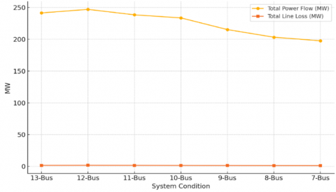
This description presents detailed power flow results under Kron Reduction on the IEEE 14-bus system. The KRM simplifies the network by eliminating buses while preserving key electrical characteristics. Each condition (from 14-Bus to 7-Bus) includes actual power flow data between bus pairs and the associated line loss. A visual summary chart shows how total line losses evolve as buses are reduced. Power flow results is shown in Table 5.

Table 5. Power flow results

Based on Table 5 can be explained, that there are values of power flow and power loss for each connecting line per condition. Total power flow and power line is shown in Figure 12.

12.jpg

Figure 12. Total power flow and power line

Based on Figure 12 can be explained, that summarizing the total power flow and line loss per condition and presenting it in a visual chart — would typically fall under the following sub-objective in a power systems research or engineering study. The results of the power flow simulation and prediction of inter-bus connection line losses.

This sub-objective concludes that system stability and voltage uniformity must be actively monitored and preserved, even in reduced models. In real-world applications, this ensures the reliability of simplified models used in real-time operation, planning, and control. This is in line with the results of Serem et al. in 2020 [46], Ranjbar et al. in 2021 [45], and Dong et al. in 2023 [44].

3.4 Determination of threshold for accuracy deterioration

One of the most important contributions of this study is identifying the threshold at which system simplification through bus reduction leads to a significant deterioration in accuracy. A critical reduction threshold was identified by comparing the total power loss, voltage profiles, and node mismatches across configurations. It was determined that reducing the system to fewer than 9 buses led to disproportionately higher errors in both voltage and loss data, signaling a tipping point in model fidelity. This threshold serves as a guideline for researchers and practitioners seeking to simplify systems without compromising simulation or control reliability.

While Kron Reduction offers an efficient way to model simplified networks, there is a critical point beyond which further reduction distorts power loss estimations, voltage profiles, and system topology integrity. This sub-objective focuses on finding that tipping point. Through systematic elimination of passive buses from the IEEE 14-bus system, multiple stages of reduction were analyzed — from the complete network down to a 7-bus configuration. At each stage, power flow simulations were run and the results compared against the original full model. Key metrics such as total power loss deviation, voltage deviation, and error propagation were monitored. Profile of power loss and voltage deviation against changes in the number of buses is shown in Figure 13, and Profile of error propagation against changes in the number of buses is shown in Figure 14.

13.jpg

Figure 13. Profile of power loss and voltage deviation against changes in the number of buses

14.jpg

Figure 14. Profile of error propagation against changes in the number of buses

Based on Figure 13 and Figure 14 can be explained, that a noticeable inflection point was observed between the 10-bus and 9-bus reductions, where deviations in both power and voltage became increasingly steep.

This threshold is crucial because it signals the boundary between acceptable and unacceptable error margins. For example, while reducing to 12 or 11 buses still maintains less than 5% deviation in power loss and voltage variance, configurations below nine buses show over 10% deviation, which may be unacceptable in critical real-time applications. These findings suggest that accuracy degradation is not linear but exponential after a specific limit is breached. Understanding this threshold in practical applications allows engineers and planners to balance computational efficiency and model fidelity. More importantly, it supports the idea that simplification should be guided by system behavior and not just structural size. This sub-objective provides actionable insight on how far simplification can be pushed before it becomes counter-productive. This is in line with the studies of Xie et al. in 2013 [47], and Ranjbar et al. in 2021 [45].

3.5 Proposal of an optimal reduction strategy

Based on the aggregated findings, an optimal strategy is proposed: reduce only non-critical passive buses that are electrically weakly connected and do not contribute significantly to power flow or system dynamics. Synthesizing all performance metrics—power loss, voltage deviation, and matrix sparsity—an optimal reduction strategy was proposed. The 10-bus and 9-bus models emerged as the most balanced configurations, achieving significant computational efficiency with minimal impact on accuracy. These models preserve essential grid dynamics, offering a practical solution for reduced-order modeling in real-time applications while maintaining a high degree of system integrity.

15.jpg

Figure 15. The illustration of trade-off between system complexity and performance

After conducting a detailed analysis of power loss, voltage profile, and accuracy thresholds, the final sub-objective focuses on proposing an optimal strategy for bus reduction. This strategy aims to simplify the power system model using Kron Reduction without compromising system reliability and computational validity. The proposed method balances three essential aspects: electrical performance, structural integrity, and analytical efficiency. The optimal strategy is based on a stepwise reduction that eliminates only passive buses while continuously evaluating power loss and voltage deviation effects. The illustration of the trade-off between system complexity and performance is shown in Figure 15.

Figure 15 explains that buses are prioritized for removal based on their connectivity, load contribution, and redundancy. For instance, low-degree buses without generation or heavy load are ideal candidates for early elimination. This ensures that the simplified model retains core electrical characteristics necessary for reliable operation.

Additionally, the strategy incorporates threshold boundaries derived from prior analyses. Any reduction step that pushes power loss or voltage deviation beyond 5-10% is considered sub-optimal and flagged for exclusion. This criteria-based approach ensures a balance between simplification and model accuracy, making it suitable for real-time monitoring, planning, or control applications. The strategy also recommends visual verification using topology diagrams and block matrices to track system structure integrity. These visual tools assist engineers in confirming that critical interconnections remain intact. When implemented, this strategy provides a reliable roadmap for reducing system complexity with minimal risk to operational accuracy, especially for large-scale smart grid environments or embedded control systems. This is in line with Dong et al. in 2023 [44], and Ranjbar et al. in 2021 [45].

While the proposed reduction strategy achieves a practical balance between computational efficiency and system performance within the IEEE 14-bus benchmark, it is essential to consider its scalability to larger power systems. Data-driven optimization approaches, although effective in structured test cases, often encounter limitations in real-world applications due to increased data complexity and computational overhead. As such, scalability remains a critical challenge. Future studies should explore how the methodology performs on larger networks and assess the integration of scalable data-driven techniques, such as machine learning-based heuristics or adaptive reduction algorithms. Addressing these challenges will be key to ensuring the robustness and applicability of the proposed approach beyond small-scale systems [2].