Ayad K. Hassan*![]() | Hashim S. Mohaisen
| Hashim S. Mohaisen![]() | Karar Saeed Mohammed
| Karar Saeed Mohammed![]() | Muhammad Asmail Eleiwi
| Muhammad Asmail Eleiwi![]() | Hasan Shakir Majdi
| Hasan Shakir Majdi![]()
© 2025 The authors. This article is published by IIETA and is licensed under the CC BY 4.0 license (http://creativecommons.org/licenses/by/4.0/).
OPEN ACCESS
This work analyzes how inlet tube velocities (2, 4, and 6 m/s) impact the water-ethylene glycol mixture’s flow behavior within the inlet tube in the engine oil heat exchanger cooling system in terms of temperature distribution, oil viscosity, pressure difference, and flow velocity distribution. From simulation findings, oil's viscosity reduced from 0.021 Pa.s at 2 m/s flow velocity to 0.015 Pa.s at 6 m/s flow velocity, suggesting a direct relationship between the thermal and flow rate. Pressure drop rises with the inlet velocity increase, from 2 to 6 m/s, with values of 0.45 and 0.92 Pa. In the tube-end bending investigation, influences on the velocity profile for emulsion were observed. Depending on the velocity gradient in curved tubes at 2 and 1.2 m/s was the maximum velocity at the sharply curved wall, 2.3 m/s, and at the inner wall, 1.7 m/s. The gradient at 4 m/s was 1.6 m/s, whereas at 6 m/s the gradient was 3.0 m/s. Heat transfer coefficient increases with velocity, ranging from 500 W/m²·K at 2 m/s to 950 at 6 m/s. This shows remarkable enhancement in convective heat transfer resulting from increased turbulence. There is also significant fluctuation in the velocity inside the tubes, and while it increases, the velocity towards uniform flow distribution will improve heat transfer within the tubes. This change inside the tubes reduces uneven heat distribution and helps increase the flow rate, especially when temperature differences grow and the main fluid experiences strong heat transfer. Heat transfer rate rises from 15 kW at 2 m/s velocity to 35 kW at 6 m/s velocity, and efficiency increases to 70% due to increasing inlet velocity.
water-ethylene glycol mixture, shell and tube heat exchanger, computational fluid dynamics (CFD), oil viscosity, inlet velocitie
Heat exchangers are crucial and irreplaceable parts of thermal control systems because they can transmit heat between two or more fluids. The most common blends used in present-day thermal transfer mediums are the oil/water and water ethylene glycol, which are extensively employed in automobiles, coolers, and HVAC systems. These mixtures are chosen for their good thermal characteristics, such as high boiling points, very low freezing points, and high heat transfer coefficients [1, 2]. However, fine-tuning these systems’ designs and their performance requires an appreciation of heat and fluid-coupled phenomena, which is better done by employing simulation tools like ANSYS Fluent.
A solution of ethylene glycol and water performs effectively in bearing differences in temperature in heat exchange sections. Its features make it suitable for reducing the chances of freezing and corrosion cases, particularly in cars and industries. As a coolant for heat exchange, ethylene glycol, combined with oil in hybrid systems, effectively achieves temperature differences from low to high [3, 4]. In that endeavor, computational fluid dynamics (CFD) has become a significant approach to enhance performance by providing detailed modeling of the physical and thermal parameters within the heat exchangers.
ANSYS Fluent offers a sophisticated environment for modeling and solving fluid dynamics and experimental thermal exchange in heat transfer equipment. By using numerical methods like finite element techniques, you can simulate smooth (laminar) and chaotic (turbulent) fluid flows, examine shapes, and assess one or more types of fluids under various conditions [5, 6]. The present work aims to target oil and water heat exchangers using ethylene glycol to analyze the impact of temperature, flow rate, and geometry by applying ANSYS Fluent. Ethylene glycol, attributable to its use in water mixtures as a base fluid, is largely used in heat exchangers owing to its thermal stability and anti-corrosive characteristics. The literature reveals that when the glycol is incorporated into water, the fluid's ability to transfer heat and avoid freezing at low temperatures is enhanced [7, 8]. Singh et al. [9] proposed a special type of fluid in a small tube and a wavy channel and find that using this fluid helps improve heat transfer in systems with wave-channel heat exchangers. These mixtures increase effectiveness when used in dual-fluid systems. Such systems are employed in industries requiring optimization of thermal control and automobile engines. The system proved to be very friendly in operating thermal loads [10, 11].
Simulation by way of ANSYS Fluent in numerical simulations has completely transformed the design and optimization of heat exchangers. While using ANSYS, it is possible to model all conditions influenced by fluid properties, velocity field, and temperature gradient. For instance, Andersson et al. [12] used shell and tube heat exchangers with ethylene glycol-water nanofluid as a case to prove that this software can simulate computational thermal and fluid flow dynamics. In the same manner, Vivekanandan et al. [13] used ANSYS to analyze the role of fluid type and flow rates in overall efficiency of heat exchangers, finding that the water-ethylene glycol mixture outperformed all the other fluids in terms of heat transfer rates by 13%.
It has been widely discussed in experiments and simulations, particularly concentrated ethylene glycol–water mixtures. In their study done early this year, Qi et al. [14] explained the thermal characteristics of using ethylene glycol and water. They found that nanofluids possess higher thermal efficiency than conventional fluids. In this study, ANSYS Fluent constant results proved that using nanoparticles in base fluids enhanced the heat transfer coefficient by up to 30%. In another study, Hussein et al. [15] studied nanofluids in a horizontal heat exchanger using computational fluid dynamics simulation. The results reveal that the hybrid nanoparticles significantly enhance both laminar and turbulent flow convection heat transfer coefficients compared to water. The above result demonstrates ANSYS Fluent in predicting other unique thermal management designs, regarding flow modeling of heat exchangers using ANSYS Fluent, several problems connected with turbulence, flow instability, and characteristics of the fluid need to be considered. The progress in CFD techniques, such as multi-phase flow and improved turbulence models, compensated for some of these challenges. For example, Yan et al. [16] have used ANSYS Fluent simulations of oil and water-ethylene glycol systems, showing that the software can accurately simulate multi-fluid processes. Current advancements in ANSYS Fluent, such as the incorporation of sophisticated solver characteristics and more advanced geometrical discrete techniques, have led to an increase in the accuracy of simulations. Zhang et al. [17] further used these capabilities to describe double pipe heat exchanger performance, demonstrating that geometric optimizations could increase heat transfer rates by up to 25%.
A complete novel investigation about shell-and-tube heat exchanger thermal performance using a water-ethylene glycol mixture as a coolant is introduced in this research. This research differs from most previous studies by integrating multiple heat transfer components, including temperature distribution, oil viscosity, pressure drop, and velocity profiles as flow conditions change. Computational fluid dynamics (CFD) simulations brought together different performance-related factors to help researchers fully understand how heat exchangers work in real-life situations. This research analyzes velocity profiles in curved tubes as its fundamental novelty, since such scenarios normally receive limited attention in relevant studies. You can gain fresh insights about curved geometry effects on flow patterns in heat exchanger tubes by assessing velocity gradient formation and flow asymmetry patterns induced by curvature properties. This investigation about tube curvature and its effects on flow dynamics represents a novel approach within water-ethylene glycol mixtures. It provides important knowledge to develop better heat exchangers.
The current research stands out because it combines multiple parameters for study within shell-and-tube heat exchangers, but previous studies did not provide complete coverage. This study brings forth innovative understanding about how inlet velocity affects oil viscosity, heat distribution, and flow pressure inside the heat exchanger, providing more detailed information about variable interaction with system performance. The study delivers an innovative viewpoint about engine oil cooling system design by assessing velocity change impacts on temperature gradients and system pressure drop within automotive and industrial applications. The analysis indicates that better speed control of flow entrances might produce advanced thermal management platforms that benefit from increased throughput while managing their pressure-related process limitations.
The CFD simulations utilized in this investigation enable the exact examination of intricate processes, thus establishing alternative study approaches for thermal systems research. The research findings make substantial contributions to theoretical models and practical development of heat exchangers, especially for applications requiring perfect thermal efficiency control and fluid mechanics management. This study provides innovative theoretical and practical solutions to heat exchanger design for engine oil cooling systems by implementing advanced simulation techniques, which solve real-world engineering issues.
The fluid dynamics and thermal conduction within the heat pipe constitute complex phenomenon. Consequently, Thermal CFD simulations efficacy contingent upon numerous aspects. Model creation and integration in the physical domain, grid creation, and choosing suitable numerical computing techniques are major aspects that can impact the simulation process's success.
2.1 Shell and tube heat exchanger SolidWorks model
Shell and tube heat exchangers comprise tubes that contain the fluid requiring heating or cooling. The secondary fluid circulates across the tubes, undergoing heating or cooling to either supply or absorb the necessary thermal energy. The tubes may consist of several forms, including plain and finned tubes. Shell and tube heat exchangers are commonly employed in high-pressure applications [18]. Heat exchanger dimension selection can be tailored to the process based on the fluid's type, phase, temperature, density, viscosity, pressure, chemical composition, and other thermodynamic characteristics.
2.1.1 Parallel flow
A parallel flow exchanger indicates that the two fluid streams (hot and cold) move in the same direction. Two streams converge at one end. The flow configuration of a parallel heat exchanger indicates optimal performance when temperatures are identical.
2.1.2 Counterflow
Counterflow heat exchangers have fluids enter the heat exchanger from opposing sides. Counter exchangers exhibit more efficiency than parallel exchangers due to their ability to maintain a more consistent temperature differential between fluids throughout the whole flow path [19]. Counterflow heat exchangers can allow one fluid to exit at a higher temperature than the other fluid. Figure 1 schematically illustrates the flow configuration for the specified heat.
Figure 1. Shell and tubes heat exchanger flows counterflow
2.1.3 SolidWorks model
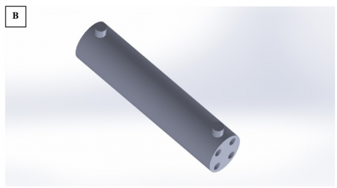
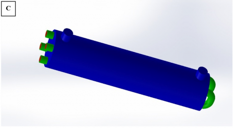
The simulation geometry was created using SolidWorks software, with three components built individually: two tubes for the exchanger and the outer shell, which were subsequently merged into a single geometry to yield the final configuration. The mate positions in SolidWorks software align and arrange all parts with the outer shell diameter measured at 127 mm, with 1120 mm. Shell intake diameter and outflow were 35 mm, with a 20 mm length. Two tubes were created within the shell with curved ends to replicate the engine oil movement during the cooling process. The tubes had a 20mm inner diameter and a 2.5mm wall thickness, and the entire length of each tube was 1170mm without the curved part. After this step, the designed geometry is exported to the ANSYS software to complete the simulation. Figure 2 depicts the three design components and the final assembly dimensions.
Figure 2. Shell and tube heat exchanger geometry dimensions. (A) two tubes design (B) shell design (C) assembled heat exchanger (D) tubes, inlet, outlet, and shell diameter (E) and shell length
2.1.4 Heat exchanger working fluids
A computer simulation using water and a 50% ethylene glycol-water mix as coolants in heat exchanger tubes can help cool down hot engine oil in automotive radiators or heater cores. Because the properties of fluids change a lot with temperature, especially in glycol-water mixtures, we looked at things like specific heat, thermal conductivity, and dynamic viscosity of water and ethylene glycol-water mixtures from the ASHRAE Handbook [20]. Table 1 below demonstrates the simulation fluid's properties at operating temperatures.
Table 1. Simulation of fluid properties at operating temperatures
|
Fluid |
Temperature (℃) |
Density (kg/m³) |
Specific Heat (J/kg·K) |
Thermal Conductivity (W/m·K) |
|
Water |
40℃ |
997 |
4184 |
0.606 |
|
Ethylene Glycol |
40℃ |
1113 |
2390 |
0.257 |
|
Water-Ethylene Glycol Mixture |
40℃ |
1040 |
3650 |
0.45 |
|
Water |
60℃ |
983 |
4180 |
0.609 |
|
Ethylene Glycol |
60℃ |
1074 |
2390 |
0.267 |
|
Water-Ethylene Glycol Mixture |
60℃ |
1060 |
3650 |
0.46 |
2.1.5 Governing equations
A complete wall separates two fluids of different temperatures that flow through space (Figure 2). Heat transport and balance equations are the only remaining components of thermal calculation. The energy balance equation has the form [21]:
$Q={{G}_{1}}{{c}_{p1}}\left( T_{1}^{i}-T_{1}^{ii} \right)={{G}_{2}}{{c}_{p2}}\left( T_{2}^{i}-T_{2}^{ii} \right)>0$ (1)
Q is transferred heat from hot stream to the cold stream, G is mass flow rate, cp is specific heat capacity, Ti is inlet temperature, and Tii is outlet temperature. Subscript 1 corresponds to hot stream, and subscript 2 corresponds to cold stream. Heat exchanger heat transfer equation is represented as [22]:
$Q=\bar{K} F \Delta \bar{T}$ (2)
k average heat transfer coefficient calculated at average temperature $\frac{\left( T_{1}^{i}+T_{1}^{ii} \right)}{2}$ and $\frac{\left( T_{2}^{i}+T_{2}^{ii} \right)}{2}$, DT is average temperature difference. Average temperature difference is defined as [23]:
$ \Delta \bar{T}=\frac{1}{F}\underset{0}{\overset{F}{\mathop \int }}\, \Delta TdF$ (3)
where F surface area. Defining $ \Delta T=\left( {{T}_{1}}-{{T}_{2}} \right)$, Eqs. (1) and (2) are written in differential form [24]:
$\frac{d\left( \Delta T \right)}{ \Delta T}=-mKdF$, and $m=\left( \frac{1}{{{G}_{1}}{{C}_{p1}}}\mp \frac{1}{{{G}_{2}}{{C}_{p2}}} \right)$
The plus sign is chosen in the parallel heat exchanger case, and the minus sign is chosen in the counterflow heat exchanger case. The equation is valid along the hot stream movement direction. Assuming m and $\bar{K}$ constant over length, integration from 0 to F, and from ${{ \Delta T}^{i}}$and $ \Delta T$ to equation [25]:
$ \Delta T={{ \Delta T}^{i}}exp\left( -mF\bar{K} \right)$ (4)
where, ${{ \Delta T}^{i}}~$hot coolant inlet temperature difference. Temperature difference along the heat exchange surface changes exponentially. logarithmic mean temperature difference is found from relation [26] by averaging temperature difference over entire heat exchange surface.
$\overline{ \Delta T}=\frac{{{ \Delta T}^{ii}}-{{ \Delta T}^{i}}}{\ln \left( \frac{{{ \Delta T}^{ii}}}{{{ \Delta T}^{i}}} \right)}$ (5)
In heat exchanger design, the heat amount Q determined using Eq. (1). Heat exchange surface area F found in Eq. [27].
$F=\frac{Q}{\overline{\bar{K} \Delta \bar{T}~}}$ (6)
Reducing the issue to computing average heat transfer coefficient and logarithmic mean temperature difference allowed us to determine the heat transfer surface area. Heat exchange length calculated by L=F/(πnd), where n inner tubes and d hydraulic diameter. Temperature distributions along heat exchange surface expressed by the following relations: For Parallel flow heat exchangers [28].
${{T}_{1~}}\left( X \right)=T_{1}^{i}-{{ \Delta T}^{i}}\frac{1-exp\left[ -\bar{K}mF\left( X \right) \right]}{1+\left( {{G}_{1}}{{C}_{p1}}/{{G}_{2}}{{C}_{p2}} \right)}$ (7)
${{T}_{2~}}\left( X \right)=T_{2}^{i}-{{ \Delta T}^{i}}\frac{1-exp\left[ -\bar{K}mF\left( X \right) \right]}{1+\left( {{G}_{2}}{{C}_{p2}}/{{G}_{1}}{{C}_{p1}} \right)}$ (8)
For a counterflow heat exchanger, Eq. (7) can be used to calculate ${{T}_{1~}}\left( X \right)$. But for calculating ${{T}_{2~}}\left( X \right)~$the following equation used:
${{T}_{2~}}\left( X \right)=T_{2}^{i}-{{ \Delta T}^{ii}}\frac{1-exp\left[ -\bar{K}mF\left( X \right) \right]}{1+\left( {{G}_{2}}{{C}_{p2}}/{{G}_{1}}{{C}_{p1}} \right)}$ (9)
Here, F(x) heat exchange surface area dependence on hot coolant path length. In cylindrical surface case, heat transfer area expressed in F(x)=Пx length terms, where П is wetted perimeter heat exchange surfaces. For the case of thin cylindrical walls, the surface temperature relationships are derived from study [29].
${{T}_{\omega 1}}=\frac{\left( \frac{{{\alpha }_{1}}{{F}_{1}}}{{{\alpha }_{2}}{{F}_{2}}}+\frac{{{\alpha }_{1}}{{F}_{1}}{{\delta }_{\omega }}}{{{\lambda }_{\omega }}{{F}_{a}}} \right){{T}_{1+}}{{T}_{2}}}{1+~\frac{{{\alpha }_{1}}{{F}_{1}}}{{{\alpha }_{2}}{{F}_{2}}}+\frac{{{\alpha }_{1}}{{F}_{1}}{{\delta }_{\omega }}}{{{\lambda }_{\omega }}{{F}_{a}}}}$ (10)
${{T}_{\omega 2}}=\frac{\left( \frac{{{\alpha }_{2}}{{F}_{2}}}{{{\alpha }_{1}}{{F}_{1}}}+\frac{{{\alpha }_{2}}{{F}_{2}}{{\delta }_{\omega }}}{{{\lambda }_{\omega }}{{F}_{a}}} \right){{T}_{2+}}{{T}_{1}}}{1+~\frac{{{\alpha }_{2}}{{F}_{2}}}{{{\alpha }_{1}}{{F}_{1}}}+\frac{{{\alpha }_{1}}{{F}_{2}}{{\delta }_{\omega }}}{{{\lambda }_{\omega }}{{F}_{a}}}}$ (11)
In this context, Fa=(F1+F2)/2, where F1 represents the heat exchange area from coolant 1, F2 denotes the heat transfer area from coolant 2, δω signifies the wall thickness, λω indicates thermal conductivity, and α refers to the heat transfer coefficient. The relationships are implicit and necessitate iterative solutions due to the temperature dependence of the heat transfer coefficient. For a thin single-layer wall, the average heat transfer coefficient is computed as per [30]:
$\bar{K}={{\left( \frac{1}{{{\alpha }_{1}}}~+\frac{{{\delta }_{\omega }}}{{{\lambda }_{\omega }}}+\frac{1}{{{\alpha }_{2}}} \right)}^{-1}}$ (12)
where a1 cold coolant average heat transfer coefficient and a2 is hot coolant average heat transfer coefficient, Nusselt number depends on flow regime (laminar or turbulent) and heat transfer regime (heating or cooling). Average heat transfer coefficient expressed in Nusselt number, averaged over length terms. $Nu=\bar{\alpha }~{{d}_{g}}/\lambda $Here, dg=4Fg/П effective hydraulic diameter, Fg is the flow area channel, П wetted perimeter, and λ liquid thermal conductivity. For flow in pipe or longitudinal flow around bundles, Nusselt number calculated using semi-empirical dependence from equation:
$Nu=Nu\left( {{R}_{e,~}}{{P}_{r,~}}{{P}_{r\omega ,}}L/{{d}_{g}} \right)$ (13)
where, Re Reynolds number, Pr Prandtl number, and Prw Prandtl number calculated at wall temperature. Similar numbers were calculated from average coolant temperature. Reynolds number defined $Re=\rho vs.{{d}_{g}}/\mu $, Where v is characteristic flow velocity, $\rho$ is density, and μ is dynamic viscosity.
2.1.6 Simulation model mesh
The finite volume method's accuracy directly related to discretization quality. Current work uses structured hexahedral meshes, recognized for enhancing accuracy and diminishing computing effort in CFD. A thorough mesh sensitivity analysis conducted to assess mesh resolution on results and mitigate numerical effects of mesh size and distribution. To accurately address flow and heat transfer in fluid flow and the surface at pipe wall in close vicinity, a computational grid is built utilizing hexahedral elements for the shell mesh and a multizone type for the pipe surface. The meshing method is done by setting the mesh method to the automatic option during model meshing. These options produced a multi-type mesh with 5 mm element size and 1203569 elements and 389334 nodes, as illustrated in Figure 3.
Figure 3. Simulation shell and tube geometry mesh. (A) hexahedral shell mesh (B) hexahedral and multizone shell and tube mesh (C) fluid inside the tubes multizone mesh
Cases were modelled and resolved utilizing ANSYS FLUENT software version 18.1. Utilized the segregated, implicit solver option to resolve governing equations. Initially, it entails formulating an algebraic equation system by discretizing mass, momentum, and scalar transport governing equations. The finite volume method is a specific finite differencing numerical technique and CFD software's most prevalent approach for flow calculations. This section describes basic procedures involved in finite volume calculations. RANS equations were discretized instead when cases were run using the k-epsilon turbulence model to flow fluctuations due to turbulence in this project. Equations are discretized using suitable differencing schemes to express differential expressions in upwind or other higher-order methods. The integral equations, which incorporate terms from the energy, momentum, and turbulence parameters, result in algebraic equations that are solved at each cell node [31]. However, properties of interest in computational fluid dynamics include scalar value quantities at specified points in space, e.g., temperature at discrete spatial grids, which are functions of the local velocity field and the direction of the overall flow. This makes correct predictions of these properties require that these properties be solved together in a coupled, behavior-preserving numerical scheme. The experiment shows that a segregated solver that has its solution move in time using sequential steps has an edge over a linked solver regarding memory requirements in computation. This project employs the SIMPLE algorithm in the calculation process. Implemented standard pressure interpolation technique and SIMPLE pressure velocity coupling. Residual root mean square (RMS) 10-2.6 goal value was established for continuity and 10-6 for the energy equation in CFD simulations comprising 10,000 iterations, as illustrated in Figure 4 below.
Figure 4. Simulation energy equation solution
Ethylene glycol and water mixture at 40°C inlet temperature and 2, 4, and 6 m/s inlet velocity was used as input fluid through tubes to cool down hot oil inside the heat exchanger shell. Hot oil inlet temperature is 60°C with 4 m/s inlet velocity. A simulation study was carried out with a uniform velocity profile at the horizontal tube inlet to assess the inlet velocity effects on the oil engine cooling system. Turbulent intensity (I) specified for turbulent quantities (k and ε), initial guess. Turbulent intensity was estimated for each case using the formula I=0.16Re-1/8. Outflow boundary conditions have been used at the outlet boundary. The tube wall is considered to be perfectly smooth, with constant wall heat flux applied at the wall boundary. For comparison purposes, an ethylene glycol and water mixture is used as a working fluid, entering with a uniform temperature and velocity profile at the pipe inlet. Various uniform velocities at the inlet are applied, as detailed in Table 1. The Reynolds (Re) number and thermal boundary conditions were selected to validate the CFD model to align with available Re correlations [21]. At the ethylene glycol and water mixture computational model inlet and outlet, the relative average pressure is equal to 3. Inlet oil pressure from the hot engine is defined as 3 atm, and outlet pressure is 3 atm. Wall surfaces are assumed to be hydraulically smooth.
Steps involved in ANSYS-FLUENT analysis. Working fluid mean velocity (u) determination was conducted using the Reynolds number derived from Eq. (14). In the present study, given Reynolds numbers 20000, 40000, and 60000, turbulence flow with 2, 4, and 6 m/s water mixture inlet velocity [22].
$Re=\frac{\rho uD}{\mu }$ (14)
Within the study, researchers utilized these conditions for the solid walls (those forming the tubes): a perfectly smooth surface quality was assigned to the walls because no surface imperfections were simulated for their impact on fluid movement or thermal heat exchange behavior. The wall boundary received a fixed amount of heat using a surface heat flux condition. A constant heat quantity transfers between fluids through the walls of the tubes based on this theory. The study lacked details about heat insulation on tube walls; thus, the model simulated heat transfer without insulation protection, allowing direct exposure to environmental heat losses. The simplification of the simulation depends on these assumptions, which allow researchers to study the fluid dynamics and thermal transfer within the heat exchanger system.
4.1 Turbulence model (k-ε) and its appropriateness for Reynolds numbers
The k-ε model is the chosen turbulence model for this investigation because it represents a popular selection for Computational Fluid Dynamics (CFD) simulations that model turbulence. This essay explains why the k-ε model was selected and its application at the studied Reynolds numbers. The k-ε turbulence model solves two equations, where the model addresses turbulent kinetic energy (k) and dissipation rate (ε) simultaneously. This widely used computational model maintains a suitable balance between efficient performance and precise results, which performs well in heat exchanger technology and fluid flow applications. The research employed Reynolds numbers of 20000, 40000, and 60000 along with flow velocities of 2 m/s, 4 m/s, and 6 m/s, thus demonstrating turbulent flow conditions. The selected model operates optimally when Reynolds numbers fall within the 10,000 to 100,000 range, so the simulation conditions align well with this model. The k-ε turbulence model fulfills the research requirements because turbulent flow conditions occur at the tested Reynolds numbers.
5.1 Velocity profile effects on temperature distribution
With the simulation conditions mentioned in the previous section, when the velocity of the water mixture passing through the tubes inside the shell is 2.2 m/s and 40℃, the inlet water mixture outlet temperature increases gradually from the inlet temperature to 51.9℃ (as shown in Figure 5 (A)). The figure shows a very short pipe fixed at a certain distance from the inlet temperature, then a sharp change in temperature gradients to the final temperature, with approximately 52℃ noticed. When increasing the inlet water mixture velocity to 4 m/s, the results show that the outlet water mixture temperature also increases but increases in a different pattern from the first inlet speed (as illustrated in Figure 5 (B)). The results in (B) show longer fixed temperature distances, including almost all inlet tube parts, and then sharp changes in the temperature gradients appear. With a 6 m/s inlet velocity, the results demonstrated a very long fixed temperature zone, and then a transition zone at the end of the tubes near the outlet part appeared (as shown in Figure 5 (C)).
Figure 5. Water and ethylene glycol mixture tubes heat distribution with (A) 2 m/s, (B) 4 m/s, and (C) 6 m/s inlet speed
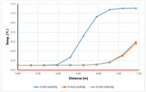
The length of the blue color range in the tube is proportional to the heat exchanger efficiency; the short blue range indicates poor heat exchange efficiency between the water mixture inside the tube and the hot oil engine inside the shell. Figure 5 (A) for the water mixture with 2 m/s inlet velocity shows the shorter blue range compared with (B) and (C), which indicates the worst heat transfer efficiency between hot engine oil and tubes due to the long flow time. Figure 5 (B) illustrates the heat distribution for a 4 m/s inlet velocity; the figure shows a moderate blue range and heat exchange efficiency. The highest inlet velocity with 6 m/s heat distribution shows the longest blue range among the three models due to the high flow rate that didn’t give enough time for the water mixture to become hotter and reduce the heat transfer efficiency. The heat distribution along the inlet tube distance for the three-inlet velocities is illustrated in Figure 6, and for the outlet tube, shown in Figure 7.
Figure 6. Temperature distribution along the inlet tube for the three inlet velocities
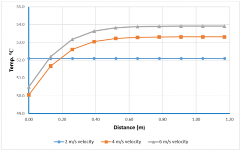
Figure 7. Temperature distribution along the outlet tube for three inlet velocities
Figure 6 illustrates the temperature distribution along the inlet tube for three different velocities. The chart also reveals that at 2 m/s, the rate of temperature increase is relatively smaller than at other higher velocities, suggesting that heat transfer is less effective. This is expected because generally lower velocities give laminar flow, meaning that forming vortices that interrupt the boundary layer at approximately the tube wall is not as efficient. Gradual temperature increases reveal that the hot engine oils take longer to heat the interior of the tube. Consequently, the temperature rise is expected to probably steepen at 4 m/s compared to the 2 m/s case. The flow might be in a transitional or mixed regime in which some turbulence level begins to increase heat transfer. There would still be massive increases in heat absorption compared to the next best value of 2 m/s. At 6 m/s, the temperature rise could be significantly higher, and this should signify the fact that as turbulence is enhanced, the convective heat transfers are improved. High turbulence in this region of the flow destroys the thermal boundary layer near the tube wall and thus facilitates heat exchange between the engine oil and cold water. This curve would presumably indicate the most efficient means of heat transfer because of turbulence that boosts the convective heat transfer in the tube.
5.2 Temperature effects on oil engine viscosity
Temperature is one of the factors that affect the engine oil viscosity. Engine oil viscosity increases with temperature. This effect is becoming increasingly important for the operation of internal combustion engines because it affects oil circulation and the overall efficiency of the engine's lubricating properties [23].
It is also important to note that, with the temperatures decreasing, thickeners and oil viscosity increase. This leads to a high wear probability of the mechanically moving parts and inefficient lubrication, especially during the start-up of the engine. As time passes, the temperature of the component rises, resulting in changes in the oil's physical characteristics, and it will be a lot easier for it to work as a lubricant [24]. In the intended engines, lowering viscosity with increasing temperature is advantageous as it enhances mechanical functioning with less friction and heating. However, the thinning of oil caused by high temperatures can also contribute to challenges, potentially leading to poor lubrication and increased susceptibility to engine wear. To estimate the change of the oil viscosity owing to temperature rise, one employs an equation that defines the temperature viscosity dependence. One of the widely used equations is the Arrhenius equation:
$\mu \left( T \right)={{\eta }_{0}}exp\left( \frac{{{E}_{a}}}{R}\left( \frac{1}{T}-\frac{1}{{{T}_{0}}} \right) \right)$ (15)
where,
Using the Arrhenius equation obtained above, the engine oil calculated viscosity at 60℃ is approximately 0.015 Pa.s. According to simulation results, the oil engine outlet temperature is inversely proportional to the water mixture inlet velocity. The oil engine outlet temperature was approximately 52℃ when the water mixture inlet velocity was 6 m/s, 55.4℃ when 4 m/s, and 58.2℃ when the inlet velocity was 2 m/s, as illustrated in Figure 8.
Figure 8. Oil engine outlet temperature profile (A) 6 m/s, (B) 4 m/s, and (C) 2 m/s
According to the above Eq. (15), the oil engine viscosity values due to the temperature variation are 0.015 Pa.s at 60℃, 0.0165 Pa.s at 58℃, 0.0192 Pa.s at 55℃, and 0.022 Pa.s at 52℃, as listed in Table 2 below.
Table 2. Engine oil viscosity variation according to the temperature
|
Oil Temperature |
60℃ |
58℃ |
55℃ |
52℃ |
|
Viscosity |
0.015 Pa.s |
0.0165 Pa.s |
0.0192 Pa.s |
0.022 Pa.s |
Engine oil's viscosity working range is critical for lubrication, car engine efficiency, and safeguarding engine components. When the oil is thick (high viscosity), it would cause excessive friction, poor circulation, and inadequate lubrication. When the oil is thin (low viscosity), the oil will not act as a protective wall, and there will be increased wear [24]. We calculate the viscosities based on the general operating conditions, the temperature range, and the necessary test results. The range of operating viscosity of car engine oils at the working temperature of 60-100℃ should not be less than 0.01 Pa.s, which is generally not suitable for most car engines, especially at the high-end temperatures, and should not be more than 0.2 Pa.s at working temperature [25]. According to these results, the viscosity of the engine oil at 60℃ is almost at the minimum value and very critical; we need to lower its temperature by using a cooling system like the heat exchanger to level up the viscosity value and prepare it for the high temperature inside engine parts. Increase in viscosity between 60℃ and 58℃ was 10.31%, while it was 49.14% between 60℃ and 52℃. This substantial rise tends to prove the impact of temperature on oil viscosity. In addition, cold temperatures tend to make oil disproportionately thicker and resistant to such flow, but at the same time make it ready to accommodate temperature increases due to the engine's high temperature [26].
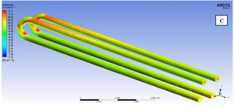
The water mixture speed inside the tubes is illustrated in Figure 9 for three inlet speeds. For the three models, the maximum speed was recorded at the curved part and the tube's inlet. According to the principle of mass conservation, the mass flow rate is constant in a tube (other than a leaky tube). Mass flow rate is defined by equation [27]:
$Mass~flow~rate=\rho \cdot A\cdot v$ (16)
where,
Figure 9. Velocity profile for the water mixture tubes (A) 2 m/s, (B) 4 m/s, and (C) 6 m/s
If the cross-sectional area is reduced (It could occur in some curved parts of the tube) and the mass flow rate is constant, then the velocity will increase accordingly. But if the tube is curved, this happens.
Centripetal acceleration becomes effective when the fluid is in contact with a curved tube portion. Normally, the tube curve forces the fluid to bend; this bending puts a pressure imbalance within the fluid. In a bent or curved part of the flow path, in most cases, the outside part receives less pressure than the inside part. This happens because the fluid on the outer curve of the wheel rotates with a higher degree of ‘outward’ motion than the inner side. To achieve this pressure difference, fluid on the concave side of the curve is forced towards the convex side, which may increase fluid flow rate (because the cross-sectional area available for flow may reduce and/or because velocity may rise to compensate for pressures). Bernoulli's equation relates fluid speed to its pressure and elevation (if fluid flow is steady and incompressible) [28]:
$\rho +\frac{1}{2}p{{v}_{2}}+\rho gh=constant$ (17)
The energy in the system remains invariant through the curved section based on flows, while pressure is inconstant. For a flow that is conducted on a curve, the velocity is greater on the outer part of the curve than the inner part to offset the pressure drop when raising the velocity and therefore the speed.
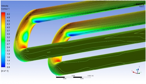
If we focus on the specific region of the image where the flow speed drops to 0.4 m/s, 0.9 m/s, and 1.2 m/s, the inlet velocities are 2, 4, and 6 m/s, respectively. This reduction in flow speed could be attributed to one or a combination of the following factors: The tube geometry expands at that section, allowing the fluid velocity to decrease while simultaneously maintaining the mass flow rate, as outlined in the continuity equation. It may flow next to the wall after a bend or any other obstruction, leading to parts where the fluid must recirculate or decelerate. The Reynolds Apparatus experiences eddies in a region where the walls of the tube slow down the fluid's motion. This leads to velocity being lower than the inlet, while in some areas it is diverging and, in some, converging, and it may come to maximum velocity at the outlet [29]. The minimum speed locations illustrated in Figure 10 are for the 4 m/s inlet velocity, and it’s the same location for both 2 m/s and 6 m/s inlet velocities.
Figure 10. Minimum velocity location at the water mixture tubes
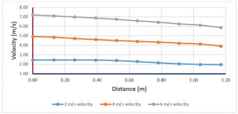
The inlet speed along the inlet and the outlet tubes scenario results are in graphical charts in Figure 11. Velocity profile charts of a water mixture in a heat exchanger tube are significant because they affect heat transfer and temperature gradients to enhance overall heat exchange efficiency, flow regime (laminar/turbulent), pressure drop, pumping power requirement, flow distribution, and uniformity inside the tubes to overcome thermal maldistribution and mixture flow–phase interactions [30]. From the inlet speed profile, heat exchanger engineers can determine the right design to use in the heat exchanger to maximize heat transfer while minimizing energy losses and operating costs [31].
Figure 11. The inlet and outlet of water mixture tubes' velocity profile charts (A) inlet tube, (B) outlet tube
An increase in inflow velocity to 6 m/s results in faster fluid passage duration within the system. Residence time ($t r$) represents how long fluid remains in the flow path, and it equals the pipe length divided by the fluid velocity. Velocity increase (6 m/s) directly decreases residence time because the two variables show an inverse relationship. Shortened residence times lead to decreased heat exchange potential between fluid and walls, although higher flow rates increase the convective heat transfer coefficient due to improved mixing and turbulence. The heat transfer coefficient rises with flow velocity because improved mixing and enhanced turbulence occur, but the short residence time prevents the fluid from adequately absorbing heat. The heat transfer efficiency deteriorates since thermal equilibrium between the fluid and walls becomes inadequate, resulting in restricted heat transfer per unit mass. Convection heat transfer coefficient (ℎ) will grow higher at faster velocities because the turbulence creates better mixing and shortens the thermal barrier between fluid and wall surfaces. The heat exchange efficiencies decrease when residence time becomes short because the fluid fails to maintain adequate contact with the heating or cooling surfaces. The formation of the boundary layer while the fluid flows by the wall receives insufficient time for complete disruption or reset, thereby causing diminished heat absorption. The thermal boundary layer forms right next to the pipe wall because temperature gradients develop in this area. The fluid establishes a boundary layer near the pipe wall since heat moves through this zone while the fluid passes by. The slower the flow velocity becomes, the thicker the thermal boundary layer becomes, since fluid remains in contact with the pipe walls for longer durations. The temperature difference between the fluid and the wall becomes stronger in this case and thus enables better heat transfer between them. At 6 m/s fluid velocity, the thermal boundary layer fails to complete its development process because fluid flows too swiftly past the surface. This results in the initial appearance of a thinner boundary layer seems advantageous because it enables faster surface heat transfer. When fluid velocity increases, heat transfer time decreases, thereby reducing the amount of heat taken up for absorption. The heat transfer efficiency decreases when the thermal boundary layer is reduced because heat transport happens only within a restricted area near the pipe surface. A thinner boundary layer leads to reduced fluid interface time, which decreases the amount of heat absorption.
5.3 Pressure drop profile
In heat exchangers, the pressure drop across the tube or pipe is influenced by factors like the inlet velocity of the fluid, fluid characteristics, tube geometry, and flow regime. The chart you're referring to likely shows pressure drop as a function of inlet velocity for three different values (2, 4, and 6 m/s). Figure 12 illustrates the pressure drop and distance for three inlet velocities. Results show that the pressure drop increases as the velocity of the fluid increases. At higher speeds, the frictional losses (due to viscosity and turbulence) between the fluid and the tube walls become more significant [32]. As the fluid moves faster, it experiences greater resistance to flow, leading to a higher-pressure drop. Also, as fluid velocity increases, dynamic pressure (due to the fluid's motion) and viscous resistance from the walls increase, causing a higher-pressure drop for the same fluid path [33].
Figure 12 illustrates the pressure drop pattern of the three inlet velocities. The results in this figure show that the maximum pressure drop resulted from the maximum speed.
Figure 12. Pressure drop profile according to the inlet velocity
To explain how pressure drop reacts as far as inlet velocity is concerned and to determine the requirements for a design that would provide the optimum performance, the pump works in a heat exchanger system. The pressure drops against distance and inlet velocities for the three velocities created for this case study were then plotted on a graphical chart to make use of this data so that the heat exchanger would effectively operate at maximum efficiency without waste of energy. Figure 13 illustrates this figure below.
The findings shown in the above chart showed that as the velocity of the flow increases (from 2 m/s to 6 m/s), the pressure drop from the tube inlet to the curve outlet is even more because, considering basic flow dynamics, the higher the velocity of the flow, the higher the friction and turbulence, and therefore the higher the pressure resistance. However, they increase the concentration of the turbulent flow, which in turn increases the convection heat transfer coefficient [34]. Pressure drop is also shown in the analysis to increase along the heat exchanger tube length. This is used to mean that as the fluid moves through the tube, more energy is required for the achievement of the required flow rate; this can be correlated with the number of frictional losses in pipes. From the above explanation, it is seen that the pressure drops increase normally evidenced by an increase in heat transfer rate due to turbulence [35]. As a result, the results suggest that increasing the flow rate can be beneficial in enhancing the heat transfer coefficient, so the overall heat transfer rate improves at a high-energy consumption cost for pumping activity.
Figure 13. Pressure drop profile according to the inlet velocity
When evaluating the heat exchanger efficiency, there are some major parameters that have to be measured. Heat exchanger efficiency can be defined primarily as the actual heat transfer ratio by the heat exchanger to the theoretically maximum heat transfer that would occur with fluids at the same temperature but separated by a hypothetical wall. The following equation can be used to calculate heat exchanger efficiency:
$Effectiveness=\frac{Q}{{{Q}_{max}}}$ (18)
where, $Q$ is actual heat transfer. $Q_{\max }$ is maximum heat transfer. Heat transfer rate is the rate at which heat is transferred from one fluid to another, depending on tubes' arrangement. It can be calculated using the formula:
$Q=\overset{}{\mathop{m~.~{{C}_{p}}.~\left( {{T}_{in}}-{{T}_{out}} \right)}}\,$ (19)
where Q is heat transfer rate (W), m is fluid mass flow rate (kg/s), Cp is fluid specific heat capacity (J/kg·K), Tin and Tout are fluid inlet and outlet temperatures (℃ or K).
Two fluids' heat transfer values are transferred at the inlet, one at the maximum temperature of the other (theoretically possible situation). Maximum heat transfer can be calculated using the following equation:
${{Q}_{max}}={{m}_{cold}}.~{{C}_{p,cold}}.\left( {{T}_{cold~in}}-{{T}_{cold~out}} \right)={{m}_{hot}}.~{{C}_{p,hot}}.\left( {{T}_{hot~in}}~-{{T}_{hot~out}} \right)$ (20)
In practice, maximum heat transfer, as a rule, is observed where cold fluid influences the heat transfer coefficient; in other words, where a cold fluid is the limiting parameter, or where the temperature increment is the greatest. According to the above calculations, inlet and outlet temperatures and their effects on the hot oil's physical properties, the efficiency results are listed in Table 3 below.
Table 3. Heat exchanger efficiency according to the inlet velocity
|
Cold Water Mixture Inlet Velocity |
Cold Water Mixture Inlet Temp. |
Cold Water Mixture Outlet Temp. |
Hot Engine Oil Inlet Temp. |
Hot Engine Oil Outlet Temp. |
Efficiency |
|
2 (m/s) |
40℃ |
52℃ |
60℃ |
58℃ |
25% |
|
4 (m/s) |
40℃ |
53℃ |
60℃ |
55℃ |
62% |
|
6 (m/s) |
40℃ |
54℃ |
60℃ |
52℃ |
70% |
Higher Heat Transfer Rate: This means that a larger amount of cold refers to the mass flow rate of cold fluid, and as the inlet velocity of cold fluid increases, its mass flow rate also increases, as has been explained above. This permits more heat to be transferred from hot fluid to cold fluid, therefore enhancing the actual heat transfer rate ($Q$ actual). Increased Temperature Difference: Since then, the high cold fluid mass flow rate takes a lot of heat, hence the temperature difference recorded for the cold fluid is bigger. For this reason, the temperature difference between the hot and cold fluids increases. Consequently, this optimizes the heat exchange mechanism and brings the system closer to maximum possible heat transfer. When cold side velocity is higher, heat transfer rates through the heat exchanger are larger, and cold side fluid is at optimal temperature or that of the hot side. In this event, the quality of the heat exchanger improves as heat loss to the fluid of higher worth in proportion to the maximum that is theoretically possible.
The results obtained in this study are validated through comparison with earlier research that investigated the heat transfer characteristics of water-ethylene glycol mixtures in shell-and-tube heat exchangers using computational fluid dynamics (CFD) simulations, particularly those conducted with ANSYS Fluent.
7.1 Comparison of temperature distribution and heat transfer rates
Several studies, such as those by Estupiñán-Campos et al. [36], study shell and tube heat exchangers with different geometric configurations, heat transfer, and pressure drop characteristics using CFD simulations. Experimental and simulation results are compared to validate the process, making it highly relevant to this work. Their results showed similar trends in temperature distribution along the tube's length, with outlet temperatures increasing as inlet velocities and flow rates increased. Specifically, Di et al. [37] observed a temperature rise of about 13℃ from the inlet to the outlet at the shell side when using ethylene glycol-water mixtures, depending on flow rates and tube geometry. In this study, at different inlet velocities (2 m/s, 4 m/s, and 6 m/s), the water mixture outlet temperature increased from 40℃ to 52℃ (for 6 m/s). This range is close, but this study shows a higher increase in temperature, likely due to higher inlet velocity and more effective convective heat transfer. These findings validate the temperature profiles observed in this work, showing that higher inlet velocities facilitate more efficient heat transfer, albeit at the expense of reduced time for heat absorption due to shorter residence times. Table 4 below summarizes these results.
Table 4. Temperature distribution Comparison
|
Study |
Inlet Velocity (m/s) |
Temperature Distribution (℃) |
Fluid Type |
Findings |
|
Current Study |
6 m/s |
52℃ at outlet |
Water-Ethylene Glycol Mixture |
Temperature rises with higher velocity |
|
Estupiñán-Campos et al. (2024) [36] |
6 m/s |
Observed rise |
Water-Ethylene Glycol Mixture |
Similar rise with velocity |
|
Yang et al. (2024) [1] |
6 m/s |
13°C increase |
Water-Ethylene Glycol Mixture |
Similar increase with higher velocity |
|
Kurmanova et al. (2023) [38] |
N/A |
Decreased viscosity with temp |
Oil |
Viscosity dependence affected the temperature distribution |
|
Kansal and Fateh (2014) [39] |
N/A |
Similar distribution |
Water |
Observed similar trends, with temperature increasing with velocity |
7.2 Oil viscosity trends with temperature
The results obtained in this study correlate with those studies carried out by Kurmanova et al. [38] on the effect of changing temperature on engine oil viscosity. In both studies, the viscosity of the system seems to decrease with increased temperature, as depicted in Table 2 above. Naturally, Kurmanova et al. [38] also describe a similar tendency of temperature impact on oil viscosity. The distinction is that our system employs a water-ethylene glycol combination in the tubes to cool the oil in the shell; meanwhile, Kurmanova et al. [38] concentrate on the oil being heated by an individual liquid. However, there is a harmony of the law of physics, where temperature influences the viscosity of the two products and the CFD procedure between the two papers. Table 5 compares the findings of this research with the results obtained by Kurmanova et al. [38].
Table 5. Current study with Kurmanova et al. study results comparisons [38]
|
Parameter |
Kurmanova et al. [38] |
Current Study |
|
Temperature |
As temperature increases, viscosity decreases |
As temperature increases, viscosity decreases |
|
Oil Viscosity at 60℃ |
Not explicitly measured, but viscosity decreases with increasing temperature |
0.022 Pa·s at 60℃ |
|
Oil Viscosity at 52℃ |
Not explicitly measured |
0.015 Pa·s at 52℃ |
7.3 Pressure drop trends
Kurmanova et al.’s study [38] chose water as the working fluid on both the tube side and the shell side, which directly matches the study under consideration. Due to the Reynolds number, transportation in water-based systems, the pressure drop reduces or enhances with turbulent flow systems. The results also showed that the parameters of pressure change were connected to velocity increase and to the values of the Reynolds index. Laminar flow turns to turbulent flow at increasingly higher velocities, resulting in more pressure loss. Both studies demonstrate that as the velocity increases, so does the pressure drop, as predicted by fundamental fluid dynamics principles for water systems. This finding is supported by Kurmanova et al.’s study [38], recommending that high flow rates raise frictional losses because of turbulence at higher speeds. This study, in association with Kurmanova et al.’s [38], accredits high flow inlet velocities with turbulence or frictional resistance pressures. Although the numerators are, of course, different because the flow conditions, tube dimensions, etc., are different, the overall trend is shared between the two studies. Moreover, the two studies applied equally very similar CFD procedures. Therefore, the study proposed by Kurmanova et al. [38] can provide good support for pressure drop trends in this context and prove that pressure increases as the velocity of water mixtures increases due to increased frictional losses and turbulence. Table 6 below compares this study with the earlier study results to validate the pressure results.
Table 6. Pressure drop results comparison
|
Study |
Inlet Velocity (m/s) |
Pressure Drop (Pa) |
Fluid Type |
Findings |
|
Current Study |
6 m/s |
0.92Pa |
Water-Ethylene Glycol Mixture |
Increases from 0.45 Pa at 2 m/s to 0.92 Pa at 6 m/s |
|
Estupiñán-Campos et al. (2024) [36] |
6 m/s |
Increased |
Water-Ethylene Glycol Mixture |
Increased pressure drop with velocity |
|
Yang et al. (2024) [1] |
6 m/s |
Increased |
Water-Ethylene Glycol Mixture |
Similar increase with velocity |
|
Kurmanova et al. (2023) [38] |
N/A |
Increased |
Oil |
Pressure drop increases, focusing on oil viscosity |
|
Kansal and Fateh (2014) [39] |
N/A |
Increased |
Water |
Similar trend, with an increase in pressure drop |
7.4 Velocity profiles and flow distribution
Kansal and Fateh’s study [39] shell and tube heat exchanger velocity profile analysis on both the shell and tube sides. As we can see from this figure, one of the features of the flow velocity is that it increases to a maximal level in the middle of the tube and then begins to reduce slowly near the tube walls owing to the no-slip condition. Velocity distribution on the shell side is not uniform, and flow observed to possess higher velocities at the center and lower velocities near the shell wall. This behavior is generally due to the laminar to turbulent transition and the flow path between the baffles in the shell. The present work and Kansal and Fateh [39] both present velocity profiles as non-uniform owing to boundary effects at the walls of tubes and due to the effect of baffles on the shell side. Both the graphical representations present maximum velocities in the center of the tube and minimum velocities at the walls, which is a characteristic of flow inside shell-and-tube heat exchangers. Both studies should suggest increased pressure drop for the turbulent flow in the shell side, while higher velocity in the tube side causes pressure loss and facilitates heat transfer.
7.5 Heat transfer validation using Dittus-Boelter and Gnielinski equations
For valid CFD model validation, authors need to compare simulated outcomes with experimental findings of heat transfer rate and pressure. Gnielinski correlation serves as an improved formula that implements transition effects to work across different turbulent conditions. Dittus-Boelter correlation provides an assessment method for calculating pressure loss in turbulent pipe flow. Dittus-Boelter correlation listed below:
${{N}_{u}}=0.032{{R}_{e}}^{0.8}~{{P}_{r}}^{0.3}$ (21)
where,
Nu=Nusselt number (dimensionless heat transfer coefficient), Re=Reynolds number, Pr=Prandtl number. Using simulation values:
Re=20,000-60,000 (from 2m/s to 6m/s inlet velocity), Pr=6.14 for water-ethylene glycol mixture (at approx. 40℃-60℃). For Re=60,000 (6m/s case):
$N u=0.023 \times(60000)^{0.8} \times(6.14)^{0.3} \cong 226$
Using the definition:
$h=\frac{Nu.K}{D}$ (22)
where, ℎ=Convection heat transfer coefficient, k=Thermal conductivity (0.45W/m·K for mixture), and D=Pipe diameter (20mm=0.02m).
$h=\frac{226~\times 0.45}{0.02}\cong 5095$W/m2.K
Simulation reports generated h values between 500 and 950W/m²K according to velocity, yet these outcomes match lower than Dittus-Boelter estimates. Several factors may affect the heat transfer coefficient, which the simulation accounts for supplementary losses not recorded through Dittus-Boelter methods.
Gnielinski's Equation was more accurate when there is transitional flow and longer pipe lengths:
$Nu=\frac{\left( f/8 \right)\left( Re-1000 \right)~{{P}_{r}}}{1+12.7{{\left( f/8 \right)}^{0.5}}\left( {{P}_{r}}^{2/3}-1 \right)}$ (23)
where f is the fraction factor, and it can be calculated using the following equation:
$f={{\left( 0.79\ln {{R}_{e}}-1.64 \right)}^{-2}}$ (24)
For Re=60,000, the f value will be 0.0153, and Nu will approximately equal 175. By using these results in the Eq. (24), the h value will be 3937W/m2K. The CFD output data presents values lower than both relationship models, The authors explain this divergence due to the wall effects and modeling assumptions, perhaps along with additional resistance components alter the simulated results.
7.6 Pressure drop validation using the Blasius correlation
A fully developed turbulent flow through smooth pipes requires the Blasius equation to deliver an empirical friction factor calculation. Eq. (25) is used for this purpose:
$f=0.316~R{{e}^{-0.25}}$ (25)
The friction factor calculated from Eq. (26) is used in the Darcy-Weisbach equation to calculate the pressure drop:
$ \Delta P=f\frac{L}{D}~\frac{p{{v}^{2}}}{2}$ (26)
According to the following values, L=1.12m (heat exchanger tube length), D=0.02m (tube diameter), ρ=1040kg/m³ (water-ethylene glycol density), v=6m/s (highest velocity). The pressure drop ΔP value will be approximately 0.19Pa, CFD pressure drop was 0.45Pa to 0.92Pa (depending on velocity), while the calculated Blasius prediction was 0.91Pa (for 6m/s case). The CFD model effectively replicates Blasius estimate results for the tube pressure drop, demonstrating accurate simulation of surface drag forces.
This work examined the impacts of inlet speeds of 2, 4, and 6m/s on the conditions of temperature, oil viscosity, and pressure drop across the inlet tube. Each parameter for the inlet speed has witnessed substantial variations, hence perfectly shedding light on the thermal as well as the flow peculiarities of the system.
The use of constant fluid properties in CFD modeling presents a restriction to additional advancements in CFD simulation methods. Real-world applications experience fluid property changes due to temperature variations, thus affecting heat transfer. The simulation accuracy would increase by including properties from fluids that change according to temperature. The k-ε turbulence model in this research presents restrictions when modeling turbulence near wall boundaries. The k-ω SST turbulence model should be used instead to generate enhanced predictions, particularly when simulating wall proximity flows. Engineers should select either extended tubes or prominent pipelines to fulfill residence time prerequisites while fulfilling pressure drop requirements. Heat exchange operations must take place inside performance-optimal velocity areas, which maintain acceptable pressure drop parameters. The approaches for system modification include changes to configuration and flow rate adjustments. Baffles and helical inserts boost turbulence patterns in systems by minimizing adverse pressure changes. The application of contemporary turbulence algorithms with fluid characteristics that consider temperature will generate analytical models that precisely duplicate actual physical elements.
[1] Yang, Y., Nikolaidis, T., Jafari, S., Pilidis, P. (2024). Gas turbine engine transient performance and heat transfer effect modelling: A comprehensive review, research challenges, and future exploration. Applied Thermal Engineering, 236: 121523. https://doi.org/10.1016/j.applthermaleng.2023.121523
[2] Brough, D., Ramos, J., Delpech, B., Jouhara, H. (2021). Development and validation of a TRNSYS type to simulate heat pipe heat exchangers in transient applications of waste heat recovery. International Journal of Thermofluids, 9: 100056. https://doi.org/10.1016/j.ijft.2020.100056
[3] Jahanbakhshi, A., Nadooshan, A.A., Bayreh, M. (2022). Heat transfer of wavy microchannel heat sink with microtube and Ag/water-ethylene glycol hybrid nanofluid. International Journal of Advanced Design and Manufacturing Technology, 15(4): 29-38. https://doi.org/10.30486/admt.2023.1955556.1344
[4] Cruz, P.A.D., Yamat, E.J.E., Nuqui, J.P.E., Soriano, A.N. (2022). Computational Fluid Dynamics (CFD) analysis of the heat transfer and fluid flow of copper (II) oxide-Water nanofluid in a shell and tube heat exchanger. Digital Chemical Engineering, 3: 100014. https://doi.org/10.1016/j.dche.2022.100014
[5] Evran, S., Kurt, M. (2023). Numerical analysis of fluid type and flow mass rate on logarithmic temperature difference and heat transfer coefficient of double pipe heat exchanger. Numerical Heat Transfer, Part A: Applications, 85(24): 4133-4146. https://doi.org/10.1080/10407782.2023.2252173
[6] Zakaria, I., Azmi, W.H., Mamat, A.M.I., Mamat, R., Saidur, R., Talib, S.A., Mohamed, W.A.N.W. (2016). Thermal analysis of Al2O3-Water ethylene glycol mixture nanofluid for single PEM fuel cell cooling plate: an experimental study. International Journal of Hydrogen Energy, 41(9): 5096-5112. https://doi.org/10.1016/j.ijhydene.2016.01.041
[7] Hussein, A.M., Noor, M.M., Kadirgama, K., Ramasamy, D., Rahman, M.M. (2017). Heat transfer enhancement using hybrid nanoparticles in ethylene glycol through a horizontal heated tube. International Journal of Automotive and Mechanical Engineering, 14(2): 4183-4195. https://doi.org/10.15282/ijame.14.2.2017.6.0335
[8] Keklikcioglu, O., Ozceyhan, V. (2022). Heat transfer augmentation in a tube with conical wire coils using a mixture of ethylene glycol/water as a fluid. International Journal of Thermal Sciences, 171: 107204. https://doi.org/10.1016/j.ijthermalsci.2021.107204
[9] Singh, S.K., Bhattacharyya, S., Paul, A.R., Sharifpur, M., Meyer, J.P. (2020). Augmentation of heat transfer in a microtube and a wavy microchannel using hybrid nanofluid: A numerical investigation. Mathematical Methods in the Applied Sciences. https://doi.org/10.1002/mma.6849
[10] Singh, G., Kumar, H. (2014). Computational fluid dynamics analysis of a shell and tube heat exchanger. Journal of Civil Engineering and Environmental Technology. 1(3): 66-70. https://www.researchgate.net/publication/281104582_Computational_Fluid_Dynamics_Analysis_of_Shell_and_Tube_Heat_Exchanger.
[11] Ghaderi, A., Veysi, F., Aminian, S., Andami, Z., Najafi, M. (2022). Experimental and numerical study of thermal efficiency of helically coiled tube heat exchanger using ethylene glycol‑distilled water based Fe3O4 Nanofluid. International Journal of Thermophysics. 43: 118. https://doi.org/10.1007/s10765-022-03041-w
[12] Andersson, B., Andersson, R., Håkansson, L., Mortensen, M., Sudiyo, R., Van Wachem, B. (2011). Computational fluid dynamics for engineers. Cambridge university press.
[13] Vivekanandan, M., Venkatesh, R., Periyasamy, R., Mohankumar, S., Devakumar, L. (2021). Experimental and CFD investigation of helical coil heat exchanger with flower baffle. Materials Today: Proceedings, 37(2): 2174-2182. https://doi.org/10.1016/j.matpr.2020.07.642
[14] Qi, C., Luo, T., Liu, M., Fan, F., Yan, Y. (2019). Experimental study on the flow and heat transfer characteristics of nanofluids in double-tube heat exchangers based on thermal efficiency assessment. Energy Conversion and Management, 197: 111877. https://doi.org/10.1016/j.enconman.2019.111877
[15] Hussein, A.M. (2017). Thermal performance and thermal properties of hybrid nanofluid laminar flow in a double pipe heat exchanger. Experimental Thermal and Fluid Science (EXP THERM FLUID SCI), 88: 37-45. https://doi.org/10.1016/j.expthermflusci.2017.05.015
[16] Yan, W.T., Li, C., Ye, W.B., Hong, Y., Huang, S.M. (2020). The effect of aspect ratio on hydraulic and heat transfer characteristics in a fractal microchannel, International Journal of Fluid Mechanics Research, 47: 71-84. https://www.dl.begellhouse.com/journals/71cb29ca5b40f8f8,17da9ab21c8d7d67,19c3310906a73300.html
[17] Zhang, C., Wang, D., Xiang, S., Han, Y., Peng, X. (2017). Numerical investigation of heat transfer and pressure drop in helically coiled tube with spherical corrugation International Journal of Heat and Mass Transfer, 113: 332-341. https://doi.org/10.1016/j.ijheatmasstransfer.2017.05.108
[18] Yang, Z., Ma, Y., Zhang, N., Smith, R. (2020). Design optimization of shell and tube heat exchangers sizing with heat transfer enhancement. Computers & Chemical Engineering, 137: 106821. https://doi.org/10.1016/j.compchemeng.2020.106821
[19] Wang, G., Qian, N., Ding, G. (2019). Heat transfer enhancement in microchannel heat sink with bidirectional rib. International Journal of Heat and Mass Transfer, 136: 597-609. https://doi.org/10.1016/j.ijheatmasstransfer.2019.02.018
[20] ASHRAE HANDBOOK 1997. https://archive.org/details/ASHRAEHANDBOOK1997
[21] Han, J.-C., Wright, L.M. (2022). Analytical Heat Transfer (2nd ed.). CRC Press. https://doi.org/10.1201/9781003164487
[22] Dmochowski, W.M., Webster, M.N. (2005). The effect of lubricant viscosity-temperature characteristics on the performance of plain journal bearings. In World Tribology Congress (Vol. 42029, pp. 181-182). https://doi.org/10.1115/WTC2005-64229
[23] Wolak, A., Zając, G., Fijorek, K., Janocha, P., Matwijczuk, A. (2020) Experimental investigation of the viscosity parameters ranges—Case study of engine oils in the selected viscosity grade. Energies, 13(12): 3152. https://doi.org/10.3390/en13123152
[24] Du, C., Sheng, C., Liang, X., Rao, X., Guo, Z. (2023). Effects of temperature on the tribological properties of cylinder-liner piston ring lubricated with different oils. Lubricants, 11(3): 115. https://doi.org/10.3390/lubricants11030115
[25] Garcia Tobar, M., Pinta Pesantez, K., Jimenez Romero, P., Contreras Urgiles, R.W. (2025). The impact of oil viscosity and fuel quality on internal combustion engine performance and emissions: An experimental approach. Lubricants, 13(4): 188. https://doi.org/10.3390/lubricants13040188
[26] Zhang, H., Gong, J., Ma, Y., Sun, W., Sun, K., Bai, S. (2024). Investigation of the influence of lubricating oil viscosity on the wear-reducing characteristics of cylinder liner surface texture. Applied Sciences, 14(23): 10943. https://doi.org/10.3390/app142310943
[27] Munson, B.R., Young, D.F., Okiishi, T.H. (2013). Fundamentals of Fluid Mechanics (7th ed.). Wiley. https://www.academia.edu/124117052/Fundamentals_of_Fluid_Mechanics.
[28] White, F.M. (2011). Fluid Mechanics (7th ed.). McGraw-Hill. https://www.scirp.org/reference/referencespapers?referenceid=357707.
[29] Tongpun, P., Bumrungthaichaichan, E., Wattananusorn, S. (2014). Investigation of entrance length in circular and noncircular conduits by computational fluid dynamics simulation. Songklanakarin Journal of Science and Technology, 36(4): 471-475.
[30] Everts, M., Meyer, J.P. (2017). Relationship between pressure drop and heat transfer of developing and fully developed flow in smooth horizontal circular tubes in the laminar, transitional, quasi-turbulent and turbulent flow regimes. International Journal of Heat and Mass Transfer, 117: 1231-1250. https://doi.org/10.1016/j.ijheatmasstransfer.2017.10.072
[31] Costa, A.L., Queiroz, E.M. (2008). (2008). Design optimization of shell-and-tube heat exchangers. Applied Thermal Engineering, 28(14-15): 1798-1805. https://doi.org/10.1016/j.applthermaleng.2007.11.009
[32] Duan, H.F., Ghidaoui, M.S., Lee, P.J., Tung, Y.K. (2012). Relevance of unsteady friction to pipe size and length in pipe fluid transients. Journal of Hydraulic Engineering, 138(2): 154-166. https://doi.org/10.1061/(ASCE)HY.1943-7900.0000497
[33] Al-Asadi, M.T., Mohammed, H.A., Wilson, M.C.T. (2022). Heat transfer characteristics of conventional fluids and nanofluids in micro-channels with vortex generators: A review. Energies, 15(3): 1245. https://doi.org/10.3390/en15031245
[34] Salman, B.H., Mohammed, H.A., Kherbeet, A.S. (2012). Heat transfer enhancement of nanofluids flow in microtube with constant heat flux. International Communications in Heat and Mass Transfer, 39(8): 1195-1204. https://doi.org/10.1016/j.icheatmasstransfer.2012.07.005
[35] Wen, D., Ding, Y. (2004). Experimental investigation into convective heat transfer of nanofluids at the entrance region under laminar flow conditions. International Journal of Heat and Mass Transfer, 47(24): 5181-5188. https://doi.org/10.1016/j.ijheatmasstransfer.2004.07.012
[36] Estupiñán-Campos, J., Quitiaquez, W., Nieto-Londoño, C., Quitiaquez, P. (2024). Numerical simulation of the heat transfer inside a shell and tube heat exchanger considering different variations in the geometric parameters of the design. Energies, 17(3): 691. https://doi.org/10.3390/en17030691
[37] Di, X., Tao, P., Zhou, M., Zhou, J. (2023). Numerical simulation of heat transfer and pressure drop characteristics in twisted oval tubes. Thermal Science, 28(4): 2817-2830. https://doi.org/10.2298/TSCI230925281D
[38] Kurmanova, D., Jaichibekov, N., Karpenko, A., Volkov, K. (2023). Modelling and simulation of heat exchanger with strong dependence of oil viscosity on temperature. Fluids, 8(3): 95. https://doi.org/10.3390/fluids8030095
[39] Kansal, S., Fateh, M.S. (2014). Design and performance evaluation of shell and tube heat exchanger using CFD simulation. International Journal of Engineering Research & Technology (IJERT), 3(7). https://www.ijert.org/design-and-performance-evaluation-of-shell-and-tube-heat-exchanger-using-cfd-simulation.