Duc Pham Xuan | Vinh Nguyen Duy*![]() | Vu Minh Dien
| Vu Minh Dien![]() | Pham Hoa Binh
| Pham Hoa Binh![]()
© 2025 The authors. This article is published by IIETA and is licensed under the CC BY 4.0 license (http://creativecommons.org/licenses/by/4.0/).
OPEN ACCESS
This paper presents an in-depth aerodynamics simulation of a prototype car utilizing computational fluid dynamics (CFD) technology. The primary objective of this research is to analyze and optimize the vehicle's aerodynamic performance to enhance its stability, efficiency, and overall performance. A detailed CFD model of the prototype car was developed, encompassing the exterior body and relevant aerodynamic features. The simulation was conducted under various operating conditions to assess the impact of different design elements on the airflow patterns, drag coefficient, and lift force. The methodology involved using advanced meshing techniques to accurately capture the complex geometries of the car and high-fidelity turbulence models to simulate the airflow dynamics. This article discusses the creation of aerodynamically optimized prototype automobile designs using examples of cars that have competed in local and international contests for fuel-efficient vehicles, such as the Shell Eco-Marathon. The designs are CFD-simulated at speeds ranging from 15 km/h to 60 km/h in 5 km/h increments. Results for drag coefficients and lift, pressure, and velocity contours are graphically shown. In addition, the results indicate significant areas for aerodynamic improvement, particularly in reducing the drag coefficient and optimizing the downforce distribution. This research contributes valuable insights into the aerodynamic design process of prototype vehicles, demonstrating the critical role of CFD technology in automotive engineering.
aerodynamics, CFD, drag coefficient, lift coefficient, drag reduction, three-dimensional
Aerodynamics plays a pivotal role among the myriad factors influencing vehicle efficiency and safety. Designing cars that minimize air resistance, optimize fuel efficiency, and maintain stability at high speeds is crucial in developing competitive and sustainable vehicles. In this context, computational fluid dynamics (CFD) technology has emerged as a powerful tool, enabling detailed simulation and analysis of aerodynamic properties without the need for costly and time-consuming physical prototypes. Only recently have automakers been more interested in low-speed aerodynamics due to the rising cost of gasoline. With the primary objective of creating clean, efficient, and sustainable cars for transportation, car makers today are focusing on making their vehicles more aerodynamic.
Due to the improved processing power available in recent years, CFD has often been used to forecast the aerodynamic flow around vehicles, making it a practical tool for modeling aerodynamic effects [1, 2]. Certain CFD software makes it simple to build up the aerodynamic properties of a complicated body near a moving wall and with moving parts, enabling real-world features to be included early in the design phase. The lattice Boltzmann approach is being employed more often in CFD solvers because of the exponential development in processing power; this has created some unrest in the Navier-Stokes-dominated CFD sector. The Navier-Stokes equations describe the fluid flow behavior. How Navier-Stokes and lattice Boltzmann computational simulations compare and contrast is still unknown.
Road vehicles' aerodynamic properties determine their energy efficiency from aerodynamic drag, safety features like crosswind stability and vehicle soiling, and how much of an impact they have on their surroundings regarding noise and air pollution. The issue is properly using them in a dynamic design environment with multiple design revisions by precisely simulating highly complicated fluid processes and obtaining findings more quickly [3]. According to previous studies, regulatory stability has caused a convergence in design, meaning that competitive circuit performance now rests on optimizing aerodynamic design [4]. This study examines the fundamentals of the aerodynamics of the car's rear backlight angle.
The CATIA simulation examined the aerodynamic behavior and the bluff body's design [5-7]. The CFD simulation is used to explore this. The investigation's model of choice focuses on the bluff body. To demonstrate the theory of the coefficient of drag and the coefficient of lift, several researchers and authors have utilized Ahmed's model, a well-known bluff body with a variety of backlight angles. For instance, Simon and Gioacchion highlighted that reference models are often used in vehicle aerodynamics research to comprehend better the flow patterns a single vehicle may provide on the road. Based on this work, they employed the Ahmad model for this investigation [8-10].
Additionally, it's important to include CFD early in the design phase to avoid later revisions and essential reworks [11]. One of the most crucial safety factors in passenger vehicles is resistance to side wind. Still, the aerodynamic efficiency of the majority of production vehicles has only ever been represented by a coefficient of drag (CD): which only depicts the vehicle's aerodynamic resistance to airflow in the forward direction [12, 13]. Additionally, models with moving ground exhibit greater aerodynamic drag during yawed flow than simulations with stable ground [14, 15].
It is generally known that when the wheels rotate, local and global aerodynamic forces are impacted [16-18]. However, designs with precise geometry employed in the construction of the vehicle provide the possibility for drag reduction early in the design process [19]. Typically, wheel and wheel cover design is only considered in the latter stages of development. Road cars often have their suspension developed apart from their aerodynamics. A moving object's ride height, pitching, and rolling moments are affected by acceleration, braking, and turning, which significantly vary in the aerodynamic coefficients [20, 21].
In recent years, high-performance computers and relatively accurate turbulence models have made CFD methods increasingly important in automotive aerodynamics research. Various studies have demonstrated the versatility and effectiveness of CFD in addressing complex aerodynamic challenges. Kabanovs et al. [22] investigated the influence of wheel, ground, and spray boundary conditions on the simulation of rear soiling of a generic SUV using CFD technology. Liu et al. [23] adopted a dynamic mesh and sliding interface to conduct a numerical simulation, investigating the transient aerodynamic characteristics of vehicles during the overtaking process under the influence of crosswinds. Keogh et al. [24] studied the aerodynamic changes that occur during cornering and the underlying physical causes of time-averaged cornering-specific flow phenomena. Cho et al. [25] used numerical simulation methods to evaluate the performance of underbody aerodynamic drag reduction devices based on the actual shape of a sedan-type vehicle. Deng et al. [26] studied the effect of the power battery pack installed in the chassis on the aerodynamic characteristics of the electric vehicle, the CFD method is used to study the flow and pressure fields of the SAE (Society of Automotive Engineers) hierarchical car model with battery packs mounted on chassis. The influence of the structure parameters of the battery pack on the automobile's aerodynamics is also analyzed in detail. Based on the simulation results, it can be seen that the battery pack installed on the chassis greatly impacts the flow and pressure field at the bottom and tail of the vehicle, causing the drag coefficient and lift coefficient to increase.
Despite significant advancements in CFD technology, numerous challenges remain in accurately predicting and optimizing the aerodynamic behavior of prototype cars. These challenges stem from the complex nature of airflow, which involves turbulent, transitional, and laminar flow regimes and the interaction between various vehicle components and the surrounding air. Addressing these issues requires sophisticated simulation techniques and a deep understanding of fluid dynamics.
With commercial software, this work intends to offer research on the aerodynamics of a prototype vehicle primarily relevant to flow analysis using CFD modeling. The goal is to utilize the knowledge of the flow to aid the stylist in enhancing the aerodynamic qualities throughout the vehicle's design. CFD is used to understand the causes of forces and moments acting on a vehicle and set goals for their controlled change rather than just anticipating the forces and moments acting on a vehicle. For CFD research, a defined process is necessary to guarantee the consistency and accuracy of simulations.
The subsequent sections will provide a detailed description of the methods employed for CFD simulation, show the outcomes of our aerodynamic study, and examine the significance of our discoveries concerning vehicle design. This paper emphasizes the significance of CFD technology in the automotive sector and its function in promoting innovation and effectiveness in vehicle development.
2.1 Geometric model
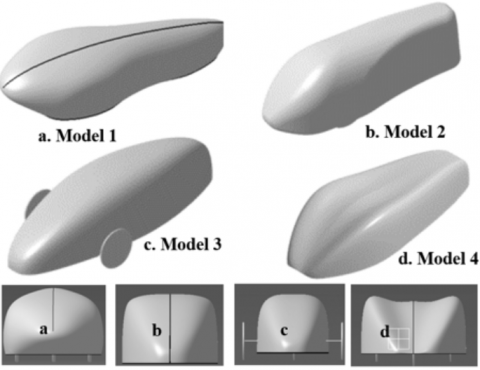
In the current research, we proposed four models of the car based on previous research and selected the best profile for the experimental procedure. The profiles and dimensions of the four models are shown in Figure 1 and Table 1.
Figure 1. Profiles of 4 simulation models
Table 1. Dimensions of simulation models
|
Model |
Length (mm) |
Width (mm) |
Height (mm) |
|
Model 1 |
2701 |
917 |
678 |
|
Model 2 |
2415 |
806 |
868 |
|
Model 3 |
2602 |
1101 |
725 |
|
Model 4 |
2665 |
1073 |
674 |
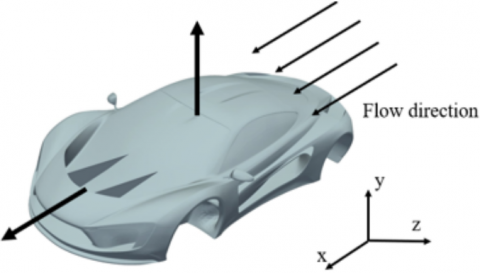
Figure 2. Drag and lift forces over a vehicle
A body immersed in a moving fluid will experience forces over its surface. The resulting force over the car in the direction of the flow, in the x-direction, is termed the drag FD. The force acting normally to this one, in the y-direction, is termed the lift FL. Figure 2 shows a representation of these two forces over a vehicle.
A side force in the z-direction, known as the side force, would be seen on the vehicle for a completely three-dimensional situation with a flow direction that is not parallel to the symmetrical plane. In addition, certain sophisticated evaluations of a vehicle's aerodynamic performance may be able to benefit from the moments these forces produce over the center of gravity of the vehicle. These moments, which revolve around the x, y, and z axes, are called rolling, jawing, and pitching moments.
Using the drag and lift coefficients is a popular strategy in fluid dynamics to handle the drag and lift force. These dimensionless numbers make it possible to measure and contrast the drag and lift of various forms. The drag coefficient (CD) is defined.
$C_D=\frac{F_D}{\frac{1}{2} \rho U^2 A}$ (1)
And the lift coefficient (CL) is defined according to:
$C_L=\frac{F_L}{\frac{1}{2} \rho U^2 A}$ (2)
where,
A: Frontal area of the object [m2]
U: Upstream velocity [m/s]
$\rho$: Density of the moving fluid [kg/m3]
As can be seen, the drag varies with density, the square of velocity, frontal area, and the dimensionless parameter CD. The form of the body has a significant impact on its drag coefficient. A car's overall drag may be decreased by decreasing the drag coefficient and area via effective aerodynamic design. In the process of designing an automobile, the product CD. A should be utilized as a guide to estimate the aerodynamic performance of the designs regardless of the fluid and velocity operating circumstances. The key objective of an efficient design would be to reduce CD and frontal area while still adhering to the dimension restrictions of the competition and the pilot's comfort. The drag increases the amount of energy required on the vehicle, decreasing its efficiency since it is one of the factors opposing the vehicle's relative movement.
2.2 Governing equations
The dominant equations for the flow representation are those from physics:
2.2.1 Equation of conservation of mass
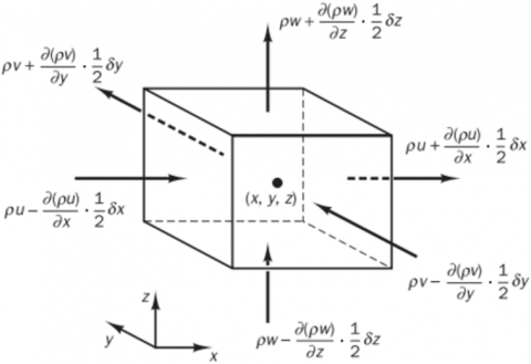
The mass of the fluid entering and leaving is permanently conserved. Let us consider a control volume of zonal, meridional, and vertical sizes $\delta_x$, $\delta_y$, and $\delta_z$ and of density $\rho$ on a fixed Cartesian coordinate system (i, j, k) attached to the ground. Mass increase in liquids is the increase in density with time:
$\frac{\partial}{\partial t}(\rho \delta x \delta y \delta z)=\frac{\partial \rho}{\partial} \delta x \delta y \delta z$ (3)
Fluid flows entering and leaving the fluid domain are shown in Figure 3.
Figure 3. Mass entering and leaving per unit volume
$\begin{aligned} & \left(\rho u-\frac{\partial(\rho u)}{\partial x} \frac{1}{2} \delta x\right) \delta y \delta z-\left(\rho u+\frac{\partial(\rho u)}{\partial x} \frac{1}{2} \delta x\right) \delta y \delta z+\left(\rho v-\frac{\partial(\rho u)}{\partial y} \frac{1}{2} \delta y\right) \delta x \delta z \\ &-\left(\rho v+\frac{\partial(\rho u)}{\partial y} \frac{1}{2} \delta y\right) \delta x \delta z+\left(\rho w-\frac{\partial(\rho w)}{\partial z} \frac{1}{2} \delta z\right) \delta x \delta y-\left(\rho w+\frac{\partial(\rho w)}{\partial z} \frac{1}{2} \delta z\right) \delta x \delta y\end{aligned}$ (4)
The mass flow rate into the element on its faces (2) equals the mass gain rate within the element. The formula is six divided by the element mass x, y, and z, and all terms of scales equal the volume of the sorted result to the left of the equal's sign. This ratio provides the continuity equation or the Equation for the conservation of mass:
$\frac{\partial \rho}{\partial t}+\frac{\partial(\rho u)}{\partial x}+\frac{\partial(\rho v)}{\partial y}+\frac{\partial(\rho w)}{\partial z}=0$ (5)
2.2.2 Equation for conservation of angular momentum
The total of the forces exerted on a fluid particle equals the rate at which its momentum increases.
According to Lagrange motion, the moment of force acting in the three directions of x, y, and z on the liquid particle is $\rho \frac{D u}{D t}$; $\rho \frac{D v}{D t}$; $\rho \frac{D w}{D t}$.
Forces acting on liquid particles:
•Mass force: Centrifugal force; Electromagnetism; Gravitation
•Facial force: Force due to pressure; Force due to viscosity
From here, we can derive the time components according to the following methods:
Direction x:
$\rho \frac{D u}{D t}=\frac{\partial\left(-p+\tau_{x x}\right)}{\partial x}+\frac{\partial \tau_{y x}}{\partial y}+\frac{\partial \tau_{z x}}{\partial z}+S_{M x}$ (6)
Direction y:
$\rho \frac{D v}{D t}=\frac{\partial \tau_{x y}}{\partial x}+\frac{\partial\left(-p+\tau_{y y}\right)}{\partial y}+\frac{\partial \tau_{z y}}{\partial z}+S_{M y}$ (7)
Direction z:
$\rho \frac{D w}{D t}=\frac{\partial \tau_{x z}}{\partial x}+\frac{\partial \tau_{y z}}{\partial y}+\frac{\partial\left(-p+\tau_{z z}\right)}{\partial z}+S_{M z}$ (8)
2.2.3. Equation of conservation of energy
The total energy gained from the waste particle equals the total heat transferred and the total work produced in the seed. Thus, the total energy increases per unit volume is $\rho \frac{D E}{D t}$.
The total heat transferred to the system is div(k*gradT). Where k is the heat transfer coefficient T is the temperature.
Total work done in liquid particles:
$\begin{gathered}{[-\operatorname{div}(p u)]+\left[\frac{\partial\left(u \tau_{x x}\right)}{\partial x}+\frac{\partial\left(u \tau_{y x}\right)}{\partial y}+\frac{\partial\left(u \tau_{z x}\right)}{\partial z}\right.}+\frac{\partial\left(v \tau_{x y}\right)}{\partial x} \\ +\frac{\partial\left(v \tau_{y y}\right)}{\partial y}+\frac{\partial\left(v \tau_{z y}\right)}{\partial z}+\frac{\partial\left(w \tau_{x z}\right)}{\partial x}\left.+\frac{\partial\left(w \tau_{y z}\right)}{\partial y}+\frac{\partial\left(w \tau_{z z}\right)}{\partial x}\right]\end{gathered}$ (9)
Thus, the energy equation can be determined:
$\begin{aligned} & \rho c \frac{D T}{D t}= \operatorname{div}(k * \operatorname{grad} T)+\tau_{x x} \frac{\partial u}{\partial x}+\tau_{y x} \frac{\partial u}{\partial y}+\tau_{z x} \frac{\partial u}{\partial z}+\tau_{x y} \frac{\partial v}{\partial x} \\ &+\tau_{y y} \frac{\partial v}{\partial y}+\tau_{z y} \frac{\partial v}{\partial z}+\tau_{x z} \frac{\partial w}{\partial x}+\tau_{y z} \frac{\partial w}{\partial y}+\tau_{z z} \frac{\partial w}{\partial z}+S_i\end{aligned}$ (10)
2.3 Boundary conditions
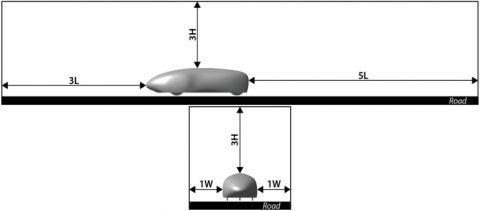
The area in space where the CFD program solves the numerical equations governing fluid flow is known as the computational domain. A computational domain size of at least two car lengths in front of the vehicle and five car lengths behind it is utilized, as advised by research on automobile exterior aerodynamics. Additionally, the simulation's vehicle was elevated by 1 centimeter. More skewed cells are formed at shorter distances between the wheels and the ground. These cells cause the solution to become unstable, which makes the problem's convergence difficult and prone to numerical mistakes. As a consequence, as shown in Figure 4, a computational domain is created to include the simulation models. The computational domain has the following dimensions: The vehicle has three car lengths in front, five car lengths behind, three car widths wide, and three car heights high.
Figure 4. Computational volume for the CFD simulations
The inlet is designated as the left border. The airflow has a velocity range of 20 to 45 km/h with 5 km/h steps. The top and right-side limits suppose an outlet pressure boundary condition. A symmetry boundary condition is considered to be the mid-vertical plane. The automobile and other barriers are seen as walls. The boundary conditions significantly impact the solution to the issue and how it is rated in math outcomes. There are several kinds of boundary conditions for traditional CFD simulations, including the following:
Airflow intake velocity: Adjust the air flow input velocity.
Gas stream outlet pressure: Adjust the gas stream outlet pressure.
Symmetry: The open domain plane is selected.
The plane is designated as the wall. Wall slip is the slip margin at the wall border condition, while wall no-slip is non-slip.
-The pressure-based simulation model is used for vehicles as the gas flow is not yet compressed, and the fundamental profile is not difficult to use owing to the low operating speed. Such research shows that $k-\varepsilon$ realizable model is more accurate than other models such as RNG, ... in free flow. Consequently, a simulation of the automobile model is run using the entangled model. Bosch's study further demonstrates that this concept is simple to set up, highly stable, and doesn't need a computer with a powerful CPU. The material selected at Material is Fluid with Air material having parameters about air density $\rho=1.225$, kinematic viscosity $\mu=1.7894 \mathrm{e}-5$.
-Set the airflow velocity and vehicle speed if the model is reversed at the boundary; the acceptable range is 15 to 60 km/h.
-The simulation type can be chosen under the Method section. Victor Fuerst Pacheco chooses the Couple solution with the best outcomes for the vehicle simulation issue based on the author's report. Research indicates that the internal technique is the best answer. Results from second-order interpolation will be superior to those from first-order interpolation.
-For automobiles, the airflow within the vehicle won't move convolutedly; therefore, you may build up 1000 interactions using Steady time.
2.4 Domain meshing
The program automatically divides the mesh of the prototype automobile. The mesh is separated into Polyhedral mesh and meshed Prims at the edge to guarantee that the behavior near the wall is estimated. Experience and study indicate that Prim's grid is often set up in 3 to 10 levels, depending on the issue and the state of the facilities already in place. This is because Prim's grid generates more components than a typical grid does. Despite requiring fewer cells to record the flow in the wake zone, it requires less processing power and memory. A fine mesh surrounding the vehicle may be able to capture flow characteristics and need less memory and processing time than a fine mesh covering the whole domain. Mesh independence research has been done to confirm mesh size does not impact the outcomes.
2.5 Setup of the problem
The simulation program offers a variety of algorithms for the solution approaches. The SIMPLE and the Coupled simulation methodologies have been employed for the simulations in this thesis. These are a few of the numerical methods for solving the discretized Navier Stokes equation that are pressure-based. The simulations were conducted using the coupled approach since it requires fewer iterations and less computing time to attain convergence. However, the SIMPLE approach was used to do the simulations when there was insufficient RAM memory.
The second-order upwind approach was used for the spatial discretization of momentum, turbulent kinetic energy, and turbulent dissipation rate. Additionally, several of the under-relaxation parameters for the momentum, pressure, turbulent viscosity, and Reynolds stress equations were modified from their default values. This was carried out regardless of whether the convergence occurred more slowly than anticipated and the stability of the solution was unaffected.
Several important variables were tracked in order to follow the iteration process, determine when it was time to end the computation, and consider whether the result converged. The continuity, the velocity components (x, y, and z): The turbulent kinetic energy, the dissipation rate, and the Reynolds stresses were first monitored using the residuals. The changes in a quantity's value between two successive iterations are known as the residuals.
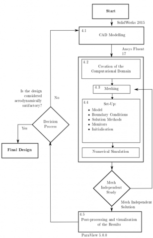
Then, a monitor for the lift and drag, which are the relevant variables, CD and CL was generated. This is the main monitor that was tracked during the iteration process, as once these values reach a steady behavior of at least the 3rd or 4rd a decimal number, the solution converged in lift and drag. If the solution was converged in terms of the drag and lift coefficients, the residual monitors were checked to ensure that all the residuals were below 10-4 or 10-5. Figure 5 shows different steps, procedures, and numerical setups.
Figure 5. Flow diagram of the simulation process
The simulation may be deemed finished, and the solution data from the whole computational volume can be exported after the convergence conditions stated have been satisfied. After processing these findings, extracting the necessary flow attributes from the calculated flow field is required. The solution yields about 100 flow parameters, such as pressure, velocity, turbulence intensity, vorticity, and an extensive list of other factors.
After simulation, the airflow through the automobile and its effects on the tire and vice versa may be seen. The post process provides tools that display velocity, pressure, and energy changes in the computational domain, where there are perturbations and vortices. The outside of the car is given a non-slip state with zero speed because of the road surface and surface.
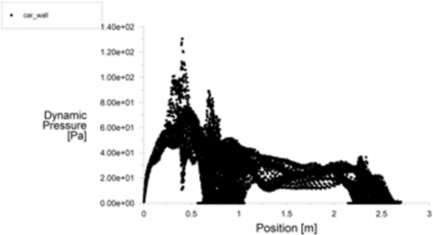
a. Model 1
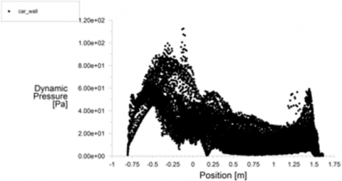
b. Model 2
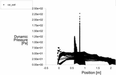
c. Model 3
d. Model 4
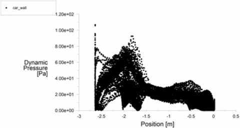
Figure 6. Dynamic pressure distribution of 4 simulation models
a. Model 1
b. Model 2
c. Model 3
d. Model 4
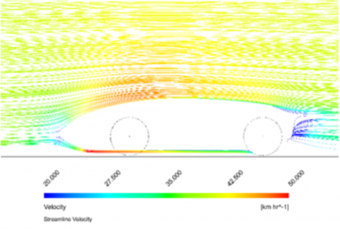
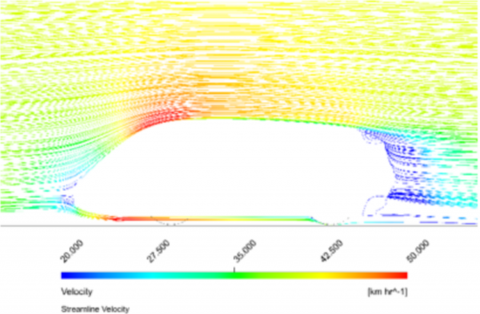
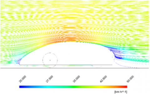
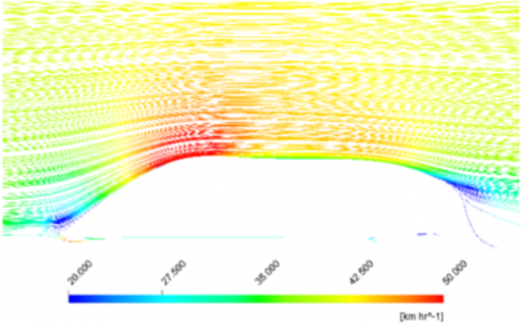
Figure 7. Comparison peed of air moving speed around the models at 40 km/h
A lifting body's lift is related to the fluid density, fluid velocity, and an associated reference area by a dimensionless lift coefficient. Aerodynamicists utilize the lift coefficient as a straightforward approach to simulate all the intricate relationships between form, tilt, and certain flow conditions and lift. This coefficient expresses the lift force to force generated by dynamic pressure times area. As shown in Figure 6 and Figure 7, the dynamic pressure and air speed are directly impacted by the aerodynamic profile, which causes a variation in the distribution of simulation models at 40 km/h. As a result, the vehicle's front end has localized zones with extremely high dynamic pressure distribution. In models 1 and 3, the dynamic pressure progressively diminishes from the front to the back of the vehicle. When there are two pressure maximums in the front and back of the vehicle in the vertical plane via the wheels, the findings in models 2 and 4 are likely to be comparable.
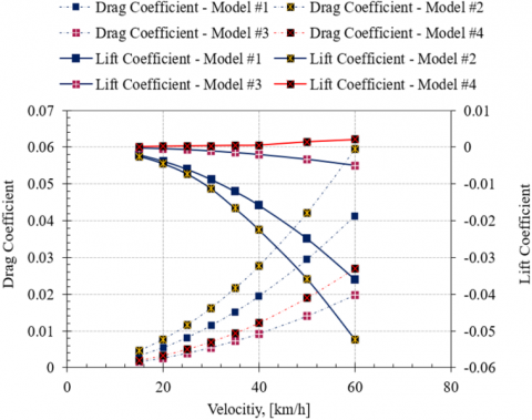
Figure 8. Comparison of the drag and lift coefficient for different models
Figure 8 compares the drag and lift coefficients for different cases. The trend in the graph shows that the lift force decreases exponentially with the increase in speed. However, there is an opposite about the drag coefficient when the drag coefficient increases with increasing velocity. For the studied profiles, the lift coefficient in ascending order is Vehicle 2, vehicle 1, vehicle 3, and Vehicle 4, respectively. Meanwhile, the drag coefficient in descending order is vehicle 2, respectively. 1, vehicle 4, and vehicle 3. The average drag coefficient of models 3 and 4 is less than 0.05 (dramatically smaller than that of other previous studies).
The results obtained from the design of Vehicle 3 and Vehicle 4 demonstrate a decrease in the aerodynamic resistance experienced by the rear wheels. The aerodynamic drag of the front wheels was decreased due to the formation of a high-pressure area at the beginning of the side air dam. However, no alterations in the flow pattern were detected when the side air dam was exclusively implemented, except for the reduction in aerodynamic drag at the wheels. However, the total aerodynamic drag increased due to the drag caused by the side air dam itself. In addition, there is a negligible disparity in the rear surface pressure between the two scenarios. The under-fin obstructed the airflow underneath the vehicle, preventing it from reaching the sides. This obstruction resulted in a decrease in aerodynamic drag around the wheels.
Additionally, the under-fin collected the airflow at the center, further reducing the micro drag in that area. Nevertheless, the decrease in the velocity of the flow underneath the vehicle's center, caused by the aerodynamic resistance of the center under-fin and the enhancement of the spreading effect in the diffuser region, resulted in a reduction in the upward flow of the air beneath the vehicle. Therefore, aerodynamic profiles 3 and 4 will be chosen to proceed with the calculating process, research, and manufacturing.
The application of CFD technology in the aerodynamic analysis of the prototype car has yielded significant insights into optimizing its design for improved performance. The simulation results underscored key areas for aerodynamic improvement, particularly in reducing the drag coefficient and optimizing the downforce distribution. This study provided a comprehensive assessment of the vehicle's aerodynamic characteristics under various operating conditions by accurately modeling the complex geometries and airflow dynamics using advanced meshing techniques and high-fidelity turbulence models. The findings demonstrated that targeted design modifications could enhance vehicle stability, efficiency, and performance. This research contributes valuable knowledge to the aerodynamic design process of prototype vehicles and highlights the indispensable role of CFD technology in advancing automotive engineering.
[1] Frink, N.T., Murphy, P.C., Atkins, H.L., Viken, S.A., Petrilli, J.L., Gopalarathnam, A., Paul, R.C. (2017). Computational aerodynamic modeling tools for aircraft loss of control. Journal of Guidance, Control, and Dynamics, 40(4): 789-803. https://doi.org/10.2514/1.G001736
[2] Natella, M., De Breuker, R. (2019). The effects of a full-aircraft aerodynamic model on the design of a tailored composite wing. CEAS Aeronautical Journal, 10: 995-1014. https://doi.org/10.1007/s13272-019-00366-5
[3] Sebben, S., Walker, T., Landström, C. (2014). Fundamentals, basic principles in road vehicle aerodynamics and design. Encyclopedia of Automotive Engineering. https://doi.org/10.1002/9781118354179.auto241
[4] Ahmed, F.S., Laghrouche, S., Mehmood, A., El Bagdouri, M. (2014). Estimation of exhaust gas aerodynamic force on the variable geometry turbocharger actuator: 1D flow model approach. Energy Conversion and Management, 84: 436-447. https://doi.org/10.1016/j.enconman.2014.03.080
[5] Watkins, S., Vino, G. (2008). The effect of vehicle spacing on the aerodynamics of a representative car shape. Journal of Wind Engineering and Industrial Aerodynamics, 96(6-7): 1232-1239. https://doi.org/10.1016/j.jweia.2007.06.042
[6] Zhou, J., Han, Q., Chen, Y. (2020). Design and analysis of the formula student car body based on CFD. In 2020 International Conference on Artificial Intelligence and Electromechanical Automation (AIEA), Tianjin, China, pp. 424-427. https://doi.org/10.1109/AIEA51086.2020.00095
[7] Guilmineau, E. (2008). Computational study of flow around a simplified car body. Journal of Wind Engineering and Industrial Aerodynamics, 96(6-7): 1207-1217. https://doi.org/10.1016/j.jweia.2007.06.041
[8] Dhaubhadel, M.N. (1996). CFD applications in the automotive industry. Journal of Fluids Engineering, 118(4): 647-653. https://doi.org/10.1115/1.2835492
[9] Hetawal, S., Gophane, M., Ajay, B.K., Mukkamala, Y. (2014). Aerodynamic study of formula SAE car. Procedia Engineering, 97: 1198-1207.https://doi.org/10.1016/j.proeng.2014.12.398
[10] Hucho, W.H., Janssen, L.J., Emmelmann, H.J. (1976). The optimization of body details—A method for reducing the areodynamic drag of road vehicles. SAE Transactions, 85: 865-882.
[11] Mayer, J., Schrefl, M., Demuth, R. (2007). On various aspects of the unsteady aerodynamic effects on cars under crosswind conditions. SAE Transactions, 116: 1463-1474.
[12] Cogotti, A. (1995). Ground effect simulation for full-scale cars in the Pininfarina wind tunnel. SAE Transactions: Journal of Passenger Cars – Mechanical Systems, 104(6): 1775–1799. https://doi.org/10.4271/950996
[13] Zhang, D., Ivanco, A., Filipi, Z. (2015). Model-based estimation of vehicle aerodynamic drag and rolling resistance. SAE International Journal of Commercial Vehicles, 8: 433-439. https://doi.org/10.4271/2015-01-2776
[14] Mayer, W., Wiedemann, J. (2007). The influence of rotating wheels on total road load. SAE Transactions, 116: 1100-1108.
[15] Maffei, M., Bianco, A. (2009). Improvements of the beamforming technique in pininfarina full scale wind tunnel by using a 3D scanning system. SAE International Journal of Materials and Manufacturing, 1: 154-168. https://doi.org/10.4271/2008-01-0405
[16] Lounsberry, T.H., Gleason, M.E., Kandasamy, S., Sbeih, K., Mann, R., Duncan, B.D. (2009). The effects of detailed tire geometry on automobile aerodynamics-a CFD correlation study in static conditions. SAE International Journal of Passenger Cars-Mechanical Systems, 2: 849-860. https://doi.org/10.4271/2009-01-0777
[17] Olsen, E., Olsson, E., Johansson, G. (1988). Vehicle aerodynamics-force and moment measurements on scaled car models using stationary and moving–belt ground planes. International Journal of Vehicle Design, 9(2): 226-241. https://doi.org/10.1504/IJVD.1988.061483
[18] Chadwick, A., Garry, K., Howell, J. (2000). Transient aerodynamic characteristics of simple vehicle shapes by the measurement of surface pressures. SAE Technical Paper, No. 2000-01-0876. https://doi.org/10.4271/2000-01-0876
[19] Mansour, H., Afify, R., Kassem, O. (2020). Three-dimensional simulation of new car profile. Fluids, 6(1): 8. https://doi.org/10.3390/fluids6010008
[20] Tan, C., Zhou, D., Chen, G., Sheridan, J., Krajnovic, S. (2020). Influences of marshalling length on the flow structure of a maglev train. International Journal of Heat and Fluid Flow, 85: 108604. https://doi.org/10.1016/j.ijheatfluidflow.2020.108604
[21] Prasad, G. (2020). Experimental and computational study of ice accretion effects on aerodynamic performance. Aircraft Engineering and Aerospace Technology, 92(6): 827-836. https://doi.org/10.1108/AEAT-03-2019-0039
[22] Kabanovs, A., Garmory, A., Passmore, M., Gaylard, A. (2019). Investigation into the dynamics of wheel spray released from a rotating tyre of a simplified vehicle model. Journal of Wind Engineering and Industrial Aerodynamics, 184: 228-246. https://doi.org/10.1016/j.jweia.2018.11.024
[23] Liu, L., Sun, Y., Chi, X., Du, G., Wang, M. (2017). Transient aerodynamic characteristics of vans overtaking in crosswinds. Journal of Wind Engineering and Industrial Aerodynamics, 170: 46-55. https://doi.org/10.1016/j.jweia.2017.07.014
[24] Keogh, J., Barber, T., Diasinos, S., Doig, G. (2016). The aerodynamic effects on a cornering Ahmed body. Journal of Wind Engineering and Industrial Aerodynamics, 154: 34-46. https://doi.org/10.1016/j.jweia.2016.04.002
[25] Cho, J., Kim, T.K., Kim, K.H., Yee, K. (2017). Comparative investigation on the aerodynamic effects of combined use of underbody drag reduction devices applied to real sedan. International Journal of Automotive Technology, 18: 959-971. https://doi.org/10.1007/s12239−017−0094−5
[26] Deng, Y., Lu, K., Liu, T., Wang, X., Shen, H., Gong, J. (2023). Numerical simulation of aerodynamic characteristics of electric vehicles with battery packs mounted on chassis. World Electric Vehicle Journal, 14(8): 216. https://doi.org/10.3390/wevj14080216