Hadeel Abdullah Mohammed* | Ahmed Abdulkadhim Hamad
© 2025 The authors. This article is published by IIETA and is licensed under the CC BY 4.0 license (http://creativecommons.org/licenses/by/4.0/).
OPEN ACCESS
Polar codes can reach the Shannon limit for an unlimited code length over a discrete memoryless channel. As an incomplete polarization process for short lengths, polar coding (PC) performs worse. Configuring the PC in a parallel or serial turbo arrangement is one way to solve this issue. The problem with turbo code is that it overestimates the information sequences sent between the parallel decoders. Consequently, a scaling factor (SF) is proposed to reduce this exaggeration, and the multiplication by SF calculated from the statistical methods increases complexity and processing time. This paper suggests a feedforward neural network (NN) with a single neuron and one hidden layer to scale the overestimating values of extrinsic information instead of multiplication by scaling factor to reduce the latency and improve the performance quality for short-length codes. Stopping criteria such as signed difference ratio (SDR) and sign change ratio (SCR) algorithms are used to avoid needless decoding iterations. In comparison to the original systematic turbo polar code (STPC), the proposed NN scaling method exhibits an enhancement of approximately 0.3 dB at BER=10-5 over AWGN noise channel. Furthermore, using stopping criteria with the proposed scheme may lower the average number of iterations (ANI) by a factor of 0.3 compared to the previous works based on the correlation coefficient approach. Furthermore, the initiation interval is reduced to one cycle using different optimization techniques like pipelining and array-partitioning.
neural network, polar codes, scaling factor, sign change ratio, signed difference ratio, systematic turbo polar codes
Arikan utilizes the polarization effect to create polar codes that can attain the symmetric channel capacity I(W). The fundamental concept of polar coding is the creation of a coding scheme that allows for individual access to one of N polarized channels,$\text{ }\!\!~\!\!\text{ }W_{N}^{\left( i \right)}$and transmits data only via channels that have a probability of error $Z\left( W_{N}^{\left( i \right)} \right)\text{ }\!\!~\!\!\text{ }$close to zero [1]. The PC has an encoder and decoder with a recursive nature and minimal complexity, making it appropriate for practical applications. For this reason, PC has attracted the interest of many researchers in the channel and source coding fields. It has also been chosen for the 5G communication [2].
The practically PC-acceptable performance is achieved at a long code length, while its performance deteriorates at a short length due to incomplete polarization of the channels$\text{ }\!\!~\!\!\text{ }W_{N}^{\left( i \right)}$. Therefore, several ways are mentioned in the literature to improve PC performance and reduce complexity, such as the pipelined architecture presented by Arikan [3]. Walaa introduces serial and parallel concatenation of turbo polar-convolutional codes to avoid short code length performance issues [4, 5]. Zhang et al. [6] used the Belief Propagation (BP) algorithm to improve PCs' performance in finite code length by applying parallel systematic polar codes. Liu et al. [7] used the BP with a soft successive cancellation list (SSCL) to achieve more enhancement. Liu et al. [8] and Qi et al. [9] employed iterative weighted decoding and punctured turbo PC to enhance PC performance. Hamad et al. [10] proposed a scaling factor (SF) estimation method of STPC with an effective early termination (ET) method based on the estimation of the correlation coefficient (CC) between a-priori ($\mathcal{P}_{k}^{t}$) and extrinsic information ($\mathcal{E}_{k}^{t}$). Deep learning (DL) algorithms that demonstrate PC's exceptional channel decoding efficiency are presented by Nachmani et al. [11] and Gruber et al. [12]. As reported by Vaz et al. [13], DL methods are investigated based on deep neural networks (DNN) for decoding PCs and recurrent neural networks (RNN) for turbo codes.
This research suggests a simple neural network (NN) with one hidden layer and a single neuron as an alternative to replace the previous SF estimation methods to enhance the performance of polar code at finite code length, reduce latency, and increase the throughput. Proposed ET schemes are the SDR [14] and SCR [15] with the STPC decoding method. The proposed scheme improves PC performance at a finite length and reduces the decoding complexity. The main contributions of this paper are summarized as follows:
The paper outlines are as follows: Section 2 reviews STPC encoding. Section 3 describes STPC decoding. The suggested NN method is introduced in Section 4. Two ET mechanisms, SCR and SDR, are presented in Section 5. The results of the simulation are demonstrated in Section 6. The conclusion of the proposed models is given in Section 7.
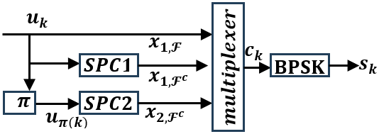
This study proposes an STPC comprising two parallel systematic polar encoders [16]. The STPC encoding process structure is illustrated in Figure 1. Encoder $i$ uses a generator matrix ${{G}_{N}}~$to produce the codeword$~{{x}_{i}}$, where, $i$=1 or 2 in the same way as any linear code. The generator matrix consists of rows of linearly independent bases. Assume that the input to the PC encoder is given by the sequence ${{u}_{k}}=\left[ {{u}_{1}},{{u}_{2}},\ldots ,{{u}_{N}} \right]$, where $u\in \left\{ 0,1 \right\}$. The output of a non-systematic PC encoder was defined by Eq. (1):
${{x}_{l}}={{u}_{l}}{{G}_{N}}={{u}_{l}}\left( {{B}_{N}}F_{2}^{\otimes n} \right)$ (1)
where, ${{B}_{N}}$ is a permutation matrix of bit-reversal in the binary field format ${{F}_{2}}$, and $\otimes n$ is the nth Kronecker product. The first kernel is given by$~{{F}^{\otimes 1}}=\left[ \begin{matrix} 1 & 0 \\ 1 & 1 \\ \end{matrix} \right]$. The data sequence is split into two parts (${{u}_{1,~\mathcal{F}}},$ ${{u}_{1,{{\mathcal{F}}^{c}})}}$ for $\mathcal{F}\subset \left\{ 1,\cdots ,N \right\}$ and ${{\mathcal{F}}^{c}}=\left\{ 1,\cdots ,N \right\}/\mathcal{F},$ where, $N$ denotes the constituent code length so that the first part ${{u}_{1,~\mathcal{F}}}$ represent the free data bits, while the second part ${{u}_{1,{{\mathcal{F}}^{c}}}}$, refer to the frozen bits. The chosen of $\mathcal{F}$ data is based on the Bhattacharyya bound approximation model [1]. Therefore, it is possible to rewrite Eq. (1) as [16, 17]:
${{x}_{1,~\mathcal{F}}}={{u}_{1,~\mathcal{F}}}{{G}_{\mathcal{F}\mathcal{F}}}+{{u}_{1,{{\mathcal{F}}^{c}}}}{{G}_{{{\mathcal{F}}^{c}}\mathcal{F}}}$ (2)
${{x}_{1,{{\mathcal{F}}^{c}}}}={{u}_{1,~\mathcal{F}}}{{G}_{\mathcal{F}{{\mathcal{F}}^{c}}}}+{{u}_{1,~{{\mathcal{F}}^{c}}}}{{G}_{{{\mathcal{F}}^{c}}{{\mathcal{F}}^{c}}}}$ (3)
${{G}_{\mathcal{F}{{\mathcal{F}}^{c}}}}$ denotes to ${{G}_{N}}$ submatrix with columns and rows indexes of ${{\mathcal{F}}^{c}}~$and $\mathcal{F}$, respectively. In systematic code, the vector ${{u}_{1,~{{\mathcal{F}}^{c}}}}$ is assigned to zero, and ${{x}_{1,~\mathcal{F}}}={{u}_{1,~\mathcal{F}}}$. Using Eq. (2) and Eq. (3), the parity bits ${{x}_{1,{{\mathcal{F}}^{c}}}}~$is given by:
${{x}_{1,{{\mathcal{F}}^{c}}}}={{x}_{1,~\mathcal{F}}}{{\left( {{G}_{\mathcal{F}\mathcal{F}}} \right)}^{-1}}{{G}_{\mathcal{F}{{\mathcal{F}}^{c}}}}$ (4)
The first encoder takes the information vector ${{u}_{k}}$ as input, while the second encoder receives the$~{{u}_{\pi \left( k \right)}}$, which is an interleaved version of ${{u}_{k}}$ to create the STPC parallel structure, as shown in Figure 1. The output of the STPC$~c=\left\{ {{x}_{1,\text{ }\!\!~\!\!\text{ }\mathcal{F}}},{{x}_{1,{{\mathcal{F}}^{c}}}},{{x}_{2,{{\mathcal{F}}^{c}}}} \right\}$ represents the overall codeword at the multiplexer output, which is constructed from systematic bits ${{x}_{1,\text{ }\!\!~\!\!\text{ }\mathcal{F}}}~$and the parity bits ${{x}_{i,{{\mathcal{F}}^{c}}}}$ generated by encoder $i$ with a total rate ${{R}_{T}}=K/{{N}_{T\text{ }\!\!~\!\!\text{ },\text{ }\!\!~\!\!\text{ }}}~$ where, ${{N}_{T}}$ refers to the total code length, and $K$ is the data length$\text{ }\!\!~\!\!\text{ }{{N}_{T}}=2N-K$. The transmitted coded bits are modulated using a binary shift-keying (BPSK) signal. The noisy data from the channel is shown in Eq. (5). Here,$\text{ }\!\!~\!\!\text{ }{{\text{ }\!\!\omega\!\!\text{ }}_{\text{k}}}$ is Gaussian noise that is spread out randomly and has a mean of zero and a variance of ${{\sigma }^{2}}={{N}_{o}}/2$,$~{{s}_{k}}=1-2{{c}_{k}}$, where, ${{s}_{k}}$ can take a value of -1 or +1 [10].
${{r}_{k}}={{s}_{k}}+{{\omega }_{k}}$ (5)
Figure 1. STPC encoder structure
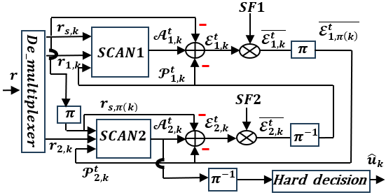
The STPC iterative decoding structure is shown in Figure 2 [16]. The decoding procedure involves the following steps:
$\mathcal{E}_{1,k}^{t}=~\mathcal{A}_{1,k}^{t}-\frac{2}{{{\sigma }^{2}}}{{r}_{s,k}}-\mathcal{P}_{1,k}^{t}$ (6)
The intrinsic information $\mathcal{I}_{1,k}^{t}$ is calculated as follows: $\mathcal{I}_{1,k}^{t}=\frac{2}{{{\sigma }^{2}}}{{r}_{s,k}}+\mathcal{P}_{1,k}^{t}$. To reduce the correlation between $\mathcal{E}_{1,k}^{t}~$and $\mathcal{I}_{1,k}^{t}$, the extrinsic is multiplied by a scaling factor represented by the symbol $SFi\le 1$, which is calculated by training a simple neural network on a dataset as mentioned in Section 4. The prior information $\mathcal{P}_{2,k}^{t}~$for SCAN-2 is generated for each iteration and is represented by Eq. (7):
$\mathcal{P}_{2,k}^{t}=\overline{\mathcal{E}_{1,\pi \left( k \right)}^{t}}$ (7)
where, $\overline{\mathcal{E}_{1,k}^{t}}=SF1\times \mathcal{E}_{1,k}^{t}$, and the symbol $\pi $ refers to the interleaving process.
Figure 2. Decoding of the STPC
$\mathcal{P}_{1,k}^{t}=\overline{\mathcal{E}_{2,.{{\pi }^{-1}}\left( k \right)}^{t}}$ (8)
Here, ${{\pi }^{-1}}$ refer to the de-interleaver, and $\overline{\mathcal{E}_{2,\text{k}}^{t}}=SF2\times \mathcal{E}_{2,k}^{t}$. Step (B) and step (C) are iterated even maximum value of iterations ${{I}_{max}}~$is achieved, or some termination technique is used to stop the iteration.
${{\hat{u}}_{k}}=\left\{ \begin{matrix} 1,~~~~~~~~~~~~~~~\mathcal{A}_{2,{{\pi }^{-1}}\left( k \right)}^{t}<0~ \\ 0,~~~~~~~~~~~~~~~~~~~~~elsewhere \\ \end{matrix} \right.$ (9)
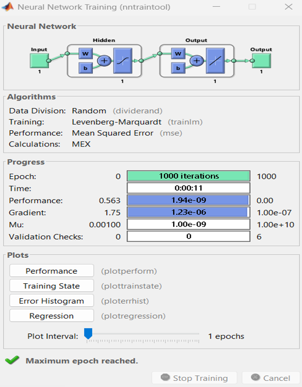
The proposed method implicitly calculates the scaling factors SF1 and SF2 using the NN technique. The optimal weights and biases are estimated from the offline training of the NN using a large dataset of optimally scaled extrinsic information obtained from the study conducted by Hamad et al. [10]. The neural networks are optimally implemented, allowing for high throughput and less utilization of resources and power. The scaled LLR sequence $\overline{\mathcal{E}_{\text{s},\text{k}}^{\text{t}}}$ is calculated by the proposed system using a single hidden layer and one neuron, as depicted in Figure 3. The equations that describe the NN are given by Eq. (10) and introduced by Havstöm and Heuts [18]:
$z=TanSig\left( \mathcal{E}_{s,k}^{t}~{{w}_{i}}+{{b}_{i}} \right)$ (10a)
$\overline{\mathcal{E}_{s,k}^{t}}=LinAct\left( z~{{w}_{o}}+{{b}_{o}} \right)$ (10b)
Figure 3. Neural network training
Table 1. Result of the training process
|
wi (Input Weight) |
bi (Output Weight) |
wo (Output Weight) |
Bo (Output Weight) |
ymin |
|
0.042 |
-0.0011 |
23.8036 |
0.0251 |
-1 |
|
xmax1 |
xmin1 |
xmax |
xmin |
ymax |
|
16.96 |
-17.7940 |
11.8720 |
-12.4560 |
1 |
Note: ymin, xmax, xmin, xmax1, xmin1, ymax are input and target normalization parameters.
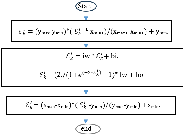
Figure 4. Scaling process by neural network
In the proposed scheme, the activation function type is the Tansigmoid ($TanSig)~$for the hidden layer, and a linear activation function ($LinAct$) for the output layer. The neuron's biases of input and output layers are$~{{b}_{i}}$ and$~{{b}_{o}}$, whereas ${{w}_{i}}$ and ${{w}_{o}}$ are the weights of hidden and output layers, respectively. The correlation coefficient method was programmed, and then the scaling factor was calculated based on the statistical equations mentioned by Hamad et al. [10], which gave optimal values. Accordingly, the values of extrinsic information before$~\mathcal{E}_{s,k}^{t} $ and after $ \overline{\mathcal{E}_{s,k}^{t}}~$scaling are stored to be used later in the training of NN. The proposed NN is training offline with a total of $64\times {{10}^{3}}$ values of $\mathcal{E}_{\text{s},\text{k}}^{\text{t}}\text{ }\!\!~\!\!\text{ }$as input and$\overline{~\mathcal{E}_{\text{s},\text{k}}^{\text{t}}}$ as the desired target, as shown in Figure 3. The optimal values of weights and bias are listed in Table 1. Figure 4 illustrates the scaling process steps of the extrinsic information values for each scan decoder.
The reliability of soft inputs and output data in conventional decoding improves with increasing iteration numbers. Unfortunately, as the number of iterations rises, the computationally complex and time-consuming processes expand [19]. The decoder performs decoding successfully before reaching the preset maximum number of iterations (Imax) for many decoding sessions, particularly at a high signal-to-noise power ratio [19]. Therefore, early termination utilization provides a practical approach to reducing computation and latency. This work uses the SDR and SCR as ET techniques to terminate extra decoding iterations in STPC_NN decoding.
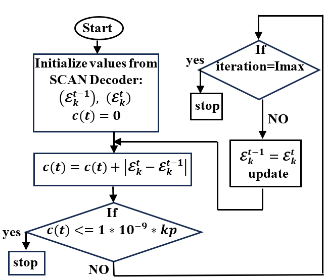
The stopping condition of the SCR depends on computing the sign changes $C\left( t \right)$ of$~\mathcal{E}_{2,k}^{t}\left( {\hat{u}} \right)$ from iteration$~\left( t-1 \right)$ to $t$ iteration. The SCR rule states that for each iteration:
$\left\{ \begin{matrix} if~C\left( t \right)<={{10}^{-9}}\times kp,~~end~the~iteration~ \\ else,~~continue~until~{{I}_{max}} \\ \end{matrix} \right.$ (11)
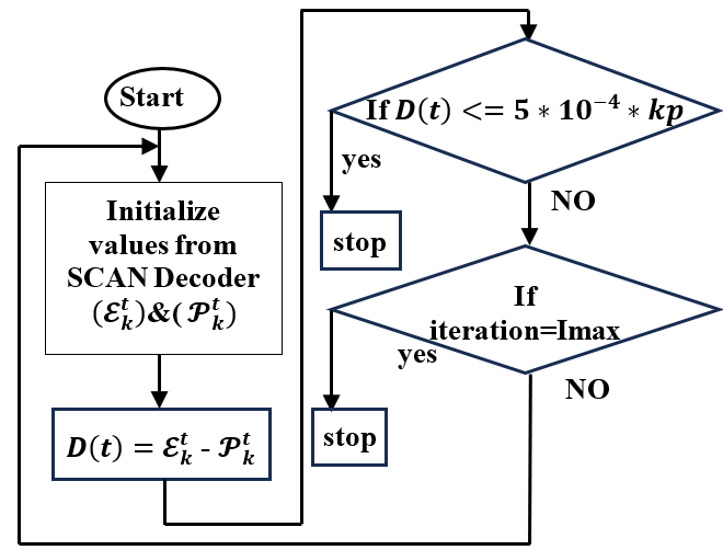
where, $kp$ is frame size. To retain the sign values of $\mathcal{E}_{2,k}^{t}\left( {\hat{u}} \right)~$from the previous iteration, the SCR approach requires a storage device, hence its complexity. This issue led to the suggestion of a different strategy known as SDR, in which for each iteration $t$, let $D\left( t \right)$ represent the number of sign differences between $\mathcal{E}_{2,k}^{t}\left( {\hat{u}} \right)$ and$~\mathcal{E}_{1,k}^{t}\left( {\hat{u}} \right)$. The condition of termination is given by Eq. (12):
$\left\{ \begin{matrix} if~D\left( t \right)\le 0.5\times {{10}^{-3}}\times kp,~~end~the~iteration~ \\ else,~~continue~until~{{I}_{max}} \\ \end{matrix} \right.$ (12)
To measure how well the current stopping criteria work, a benchmark ET technique called the "Genie stopping rule" is simulated [20]. Genie assumes that the decoder is believed to have complete knowledge about the communicated bits and finishes decoding if the rule in Eq. (13) is satisfied:
$\left\{ \begin{matrix} if~{{{\hat{u}}}_{k}}={{u}_{k}}~for~all~k~bits,~~end~the~iteration~ \\ else,~~continue~until~{{I}_{max}} \\ \end{matrix} \right.$ (13)
The simulated steps of the SDR and SCR algorithms are summarized in Figure 5.
(a)
(b)
Figure 5. Early terminations criteria: (a) SDR; (b) SCR
In this study, MATLAB R2020b was utilized to compare the performance of proposed techniques against decoding methods [4, 10]. The STPC-NN-SDR and STPC-NN-SCR codes were tested by examining their bit error rate (BER) and frame error rate (FER) performance over AWGN. The specific parameters of the proposed STPC systems are detailed in Table 2.
Table 2. Proposed parameter values
|
Parameter |
Value |
|
The frame size of NN training |
64 |
|
The data length of STPC (K) |
64, 128 |
|
Rate of constituent PC |
1/2 |
|
STPC rate |
1/3, 1/2 |
|
Number of NN frame training |
1000 |
|
Modulation type |
BPSK |
|
The PC construction method |
Bhattacharya |
|
Constituent decoders type |
SCAN |
|
Maximum iteration Imax |
6 |
|
Minimum block errors |
100 |
|
Channel type |
AWGN, $\mathcal{N}\left( 0,{{\sigma }^{2}} \right)$, ${{\sigma }^{2}}=1/\left( 2{{R}_{T}}{{E}_{b}}/{{N}_{o}} \right)$ |
|
Maximum number of block samples |
1,000,000 |
|
Minimum number of block samples |
50,000 |
(a)
(b)
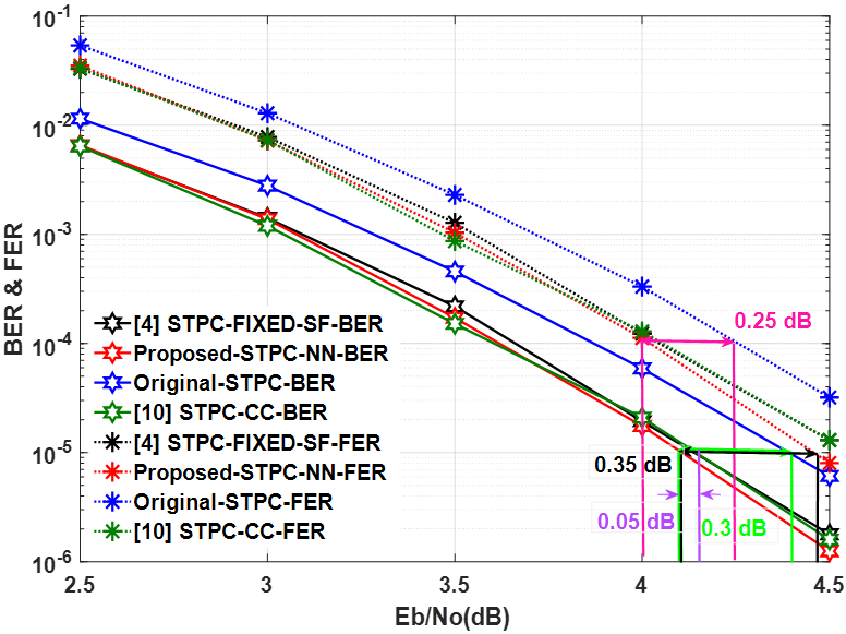
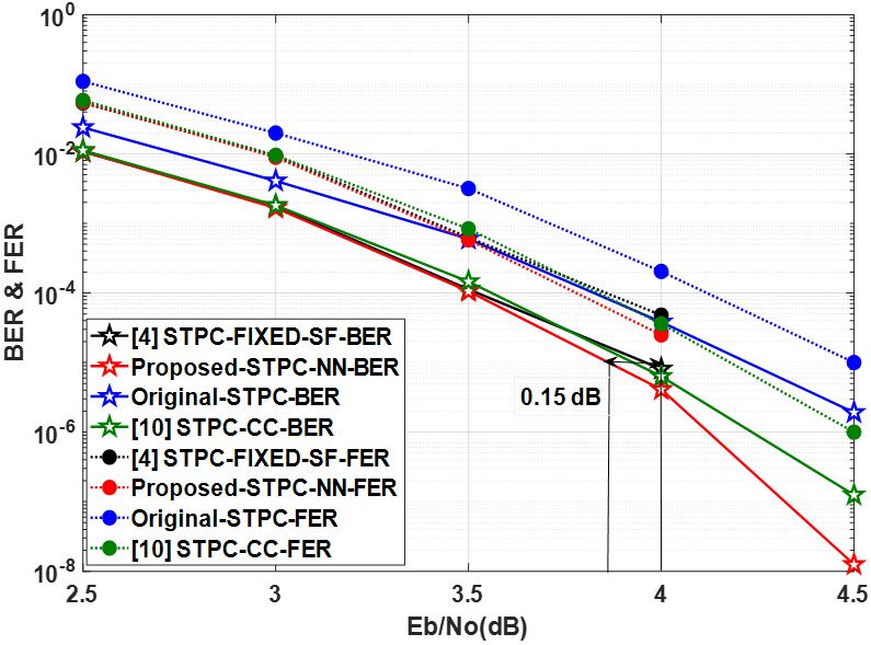
Figure 6. BER performance of different STPC schemes with ${{I}_{max~}}$=6, rate 1/3: (a) K=64; (b) K=128
6.1 Simulation results with fixed iterations
This section presents the results of simulated STPC systems with six decoding iterations. A performance comparison in terms of BER and FER against$~{{E}_{b}}/{{N}_{o}}$ for the proposed STPC-NN that employs a neural network, the STPC-Fixed-SF presented by Alebady and Hamad [4] and STPC-CC scheme utilizes an adaptive scaling factor offered by Hamad et al. [10], depicted in Figure 6 for k=64 and 128, R=1/3, R=1/2 respectively. Additionally, the original STPC system without SF is simulated as a reference to highlight the benefits of the proposed weighted scheme. At BER and FER of$~{{10}^{-5}}$, the STPC-NN shows a 0.3 dB and 0.25 dB enhancement, respectively, over the original STPC without scaling factors. It also slightly outperforms the STPC-CC and STPC-Fixed-SF by approximately 0.05 dB. For the same parameter the STPC-CC system with code length N=256 bit found that the STPC-NN exceed the STPC-CC by 0.15 dB at BER=$~{{10}^{-6}}$.
6.2 Complexity analysis result
High-level synthesis (HLS Vitis 2022.1) was utilized to assess the latency and utilization improvement of the proposed scheme. All systems are designed based on the Genesys 2 board, which has a Kintex-7 Field Programmable Gate Array (FPGA) and a core part number XC7K325T-2FFG900C. Table 3 illustrates the design schemes with and without applying pipeline using directive pragma offered by the HLS Vitis platform. The optimized schemes enhance the time delay at the expense of increasing the required resources.
Table 3. Delay and utilization analysis
|
Parameter |
Proposed NN |
CC [10] |
||
|
Without Pipeline |
With Pipeline |
With Pipeline +Array Partitioning |
With Pipeline |
|
|
Latency (cycles) |
6209 |
323 |
93 |
839 |
|
Interval (cycles) |
6210 |
324 |
1 |
840 |
|
BRAM_18K |
0 |
0 |
0 |
0 |
|
DSP |
15 |
55 |
2688 |
913 |
|
FF |
1620 |
9702 |
243166 |
116034 |
|
LUT |
2665 |
8827 |
255682 |
87628 |
Table 3 reveals that the proposed NN scheme has reduced latency, interval, and utilization of the pipeline technique compared to CC. If the array partitioning pragma is added, even 1 cycle (10 ns) can be reached in every scaling process with an N sequence of extrinsic information at the expense of increased resources.
6.3 Results of STPC with early termination
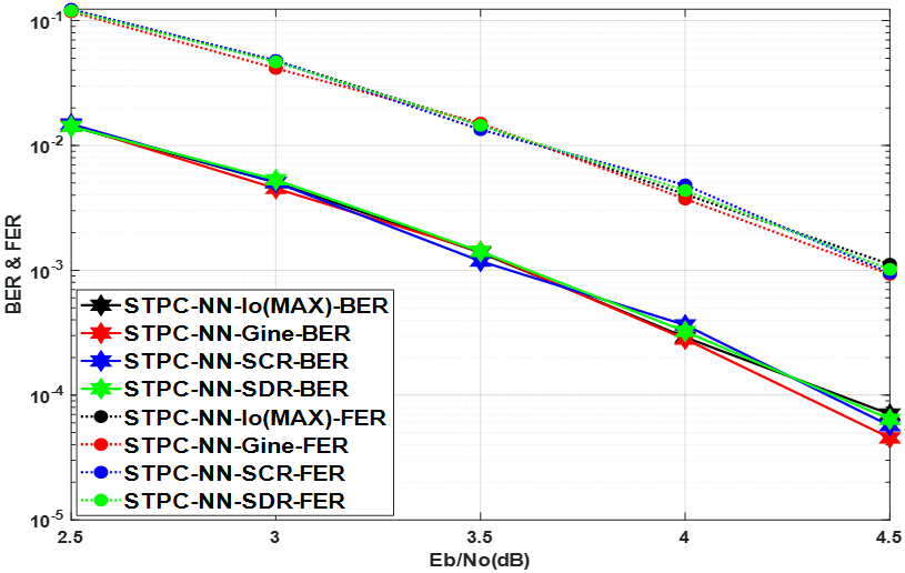
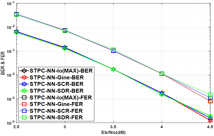
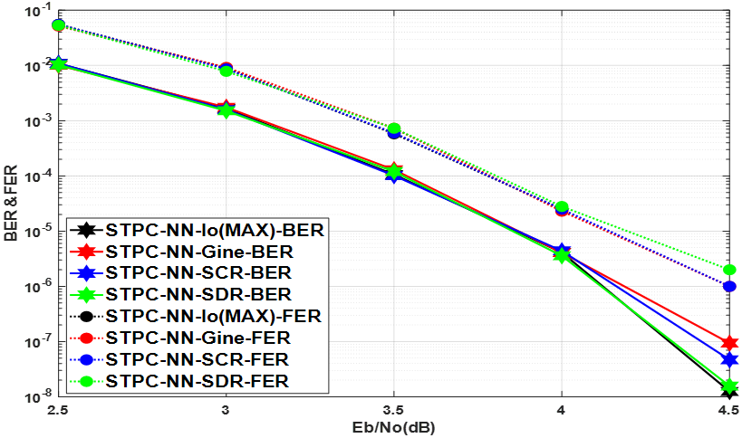
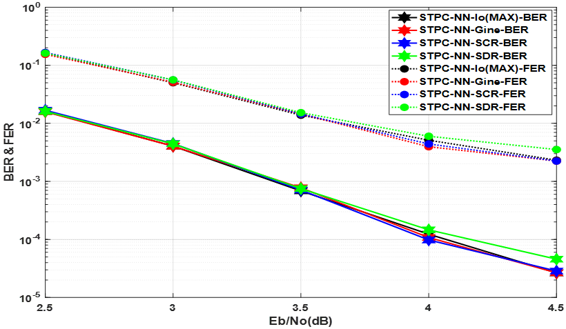
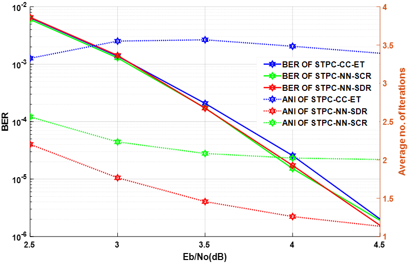
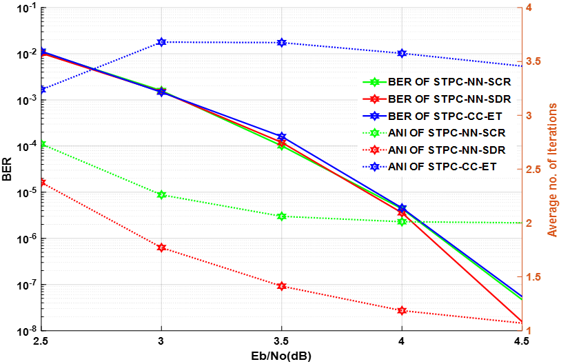
Several simulation experiments were run to illustrate the impact of ET on the proposed performance. Figures 7 and 8 demonstrate the proposed system (STPC-NN) using a neural network with SDR (STPC-NN-SDR), SCR (STPC-NN-SCR), and GINE (STPC-NN-Gine) ET techniques for K=64 and 128 with different turbo coding rates (1/2 and 1/3). The simulation tests for various systems show a comparative performance.
Figure 9 compares the proposed system with the method studied by Hamad et al. [10] regarding the average number of iterations (ANI). The proposed schemes, STPC-NN-SDR and STPC-NN-SCR, reduce the required ANI compared to STPC-CC-ET by approximately 70% and 41%, respectively. These ANI reductions without compromising performance suggest improved data throughput and lower latency.
(a)
(b)
Figure 7. STPC-NN results of K=64 with different ET: (a) R=1/3; (b) R=1/2
(a)
(b)
Figure 8. STPC-NN results with different ET at K=128: (a) R=1/3; (b) R=1/2
(a)
(b)
Figure 9. ANI of the suggested STPC with an early termination: (a) K=64; (b) K=128
This research presents a new approach to tackle the performance degradation of PCs at short lengths and alleviate the overestimation issue when constructing them in a turbo decoding scheme. The proposed solution involved a simple neural network with one hidden layer and a single neuron, which effectively replaces the conventional scaling techniques, thereby reducing complexity, power consumption, and processing delay in hardware implementation. Furthermore, the employing of stopping criteria such as signed difference ratio (SDR) and sign change ratio (SCR) algorithms significantly improve the decoding efficiency of the proposed scheme in terms of the average number of iterations (ANI) as compared with the system adopted by Hamad et al. [10]. The results suggest promising prospects for deploying neural network-based scaling schemes and stopping criteria to enhance PC communication systems' efficiency and reliability. For future work, testing NN with different parameters are interesting. Different ET mechanisms like Cross-entropy or threshold static methods can be applied.
[1] Arikan, E. (2009). Channel polarization: A method for constructing capacity-achieving codes for symmetric binary-input memoryless channels. IEEE Transactions on Information Theory, 55(7): 3051-3073. https://doi.org/10.1109/TIT.2009.2021379
[2] Bioglio, V., Condo, C., Land, I. (2020). Design of polar codes in 5G new radio. IEEE Communications Surveys & Tutorials, 23(1): 29-40. https://doi.org/10.1109/COMST.2020.2967127
[3] Arıkan, E. (2010). Polar codes: A pipelined implementation. In Proceedings 4th International Sympathetic Broad Communication, pp. 11-14. https://hdl.handle.net/20.500.14371/3610.
[4] Alebady, W.Y., Hamad, A.A. (2023). Concatenated turbo polar-convolutional codes based on soft cancellation algorithm. Physical Communication, 58: 102010. https://doi.org/10.1016/j.phycom.2023.102010
[5] Alebady, W.Y., Hamad, A.A. (2022). Turbo polar code based on soft-cancelation algorithm. Indonesian Journal of Electrical Engineering and Computer Science, 26(1): 521-530. https://doi.org/10.11591/ijeecs.v26.i1.pp521-530
[6] Zhang, Q., Liu, A., Zhang, Y., Liang, X. (2015). Practical design and decoding of parallel concatenated structure for systematic polar codes. IEEE Transactions on Communications, 64(2): 456-466. https://doi.org/10.1109/TCOMM.2015.2502246
[7] Liu, Z., Niu, K., Lin, J. (2017). Parallel concatenated systematic polar code based on soft successive cancellation list decoding. In 2017 20th International Symposium on Wireless Personal Multimedia Communications (WPMC), Bali, Indonesia, pp. 181-184. https://doi.org/10.1109/WPMC.2017.8301804
[8] Liu, Z.Z., Niu, K., Lin, J.R., Sun, J.Y., Guan, H. (2018). Scaling factor optimization of turbo-polar iterative decoding. China Communications, 15(6): 169-177. https://doi.org/10.1109/CC.2018.8398513
[9] Qi, Y., Chen, D., Zhang, C. (2019). Punctured turbo-polar codes. In 2019 IEEE 11th International Conference on Communication Software and Networks (ICCSN), Chongqing, China, pp. 736-741. https://doi.org/10.1109/ICCSN.2019.8905352
[10] Hamad, A.A., Gatte, M.T., Abdul-Rahaim, L.A. (2023). Efficient systematic turbo polar decoding based on optimized scaling factor and early termination mechanism. International Journal of Electrical and Computer Engineering (IJECE), 13(1): 629-637. https://doi.org/10.11591/ijece.v13i1.pp629-637
[11] Nachmani, E., Be'ery, Y., Burshtein, D. (2016). Learning to decode linear codes using deep learning. In 2016 54th Annual Allerton Conference on Communication, Control, and Computing (Allerton), Monticello, USA, pp. 341-346. https://doi.org/10.1109/ALLERTON.2016.7852251
[12] Gruber, T., Cammerer, S., Hoydis, J., Ten Brink, S. (2017). On deep learning-based channel decoding. In 2017 51st Annual Conference on Information Sciences and Systems (CISS), Baltimore, USA, pp. 1-6. https://doi.org/10.1109/CISS.2017.7926071
[13] Vaz, A.C., Nayak, C.G., Nayak, D., Hegde, N.T. (2022). Decoding of turbo code and polar code using deep learning for visible light communication. Journal of Engineering Science and Technology, 17(4): 2776-2787.
[14] Wu, Y., Woerner, B.D., Ebel, W.J. (2000). A simple stopping criterion for turbo decoding. IEEE Communications Letters, 4(8): 258-260. https://doi.org/10.1109/4234.864187
[15] Shao, R.Y., Lin, S., Fossorier, M.P. (1999). Two simple stopping criteria for turbo decoding. IEEE Transactions on Communications, 47(8): 1117-1120. https://doi.org/10.1109/26.780444
[16] Wu, D., Liu, A., Zhang, Y., Zhang, Q. (2016). Parallel concatenated systematic polar codes. Electronics Letters, 52(1): 43-45. https://doi.org/10.1049/el.2015.2592
[17] Wang, X.M., Li, J., Wu, Z.T., He, J.L., Zhang, Y., Shan, L. (2020). Improved NSC decoding algorithm for polar codes based on multi-in-one neural network. Computers & Electrical Engineering, 86: 106758. https://doi.org/10.1016/j.compeleceng.2020.106758
[18] Havstöm, P., Heuts, O. (2023). Machine Learning Assisted Quantum Error Correction Using Scalable Neural Network Decoders. http://hdl.handle.net/20.500.12380/305996.
[19] Kim, B., Lee, H.S. (1999). Reduction of the number of iterations in turbo decoding using extrinsic information. In Proceedings of IEEE Region 10 Conference. TENCON 99.'Multimedia Technology for Asia-Pacific Information Infrastructure', Cheju, Korea (South), pp. 494-497. https://doi.org/10.1109/TENCON.1999.818459
[20] Obiedat, E.A., Cao, L. (2008). Turbo decoder for low-power ultrawideband communication systems. International Journal of Digital Multimedia Broadcasting, 2008(1): 897069. https://doi.org/10.1155/2008/897069