Sabah H. Alwan*![]() | Ali K. Jasim
| Ali K. Jasim![]() | Yasser F. Hasan
| Yasser F. Hasan![]()
© 2023 IIETA. This article is published by IIETA and is licensed under the CC BY 4.0 license (http://creativecommons.org/licenses/by/4.0/).
OPEN ACCESS
In the field of power transmission, underground cables are subjected to various factors that influence their load capacity. One such significant factor, often overlooked, is the extreme environmental conditions prevalent in certain geographical regions. This study particularly focuses on regions where summer temperatures exceed 50℃ and the soil, due to excessive dryness, exhibits high thermal resistivity. The current study explores the impact of these harsh environmental conditions on the current-carrying capacity (ampacity) of underground power cables. A derating factor for dry zone formation around these cables has been proposed, calculated for various types of native soil. The standard IEC-60287 has been adhered to as a reference for these calculations. The software ANSYS has been employed to compute the temperature distribution around the cables in different types of soil, using relevant experimental data. The results indicate that the formation of dry regions in the soil begins at differing temperatures and rates depending on the soil's composition. This study thus underscores the critical role of environmental factors and soil conditions in determining the ampacity of underground power cables. It also highlights the necessity of incorporating these factors into design considerations for optimal cable performance.
ANSYS software, life expectancy, temperature distribution, dry zone, underground cables, harsh environment
In general, PVC insulations are affected basically by thermal stress as well as mechanical stress in low voltage applications: therefore, the conductor temperature under loading conditions must be less than or equal the nominal temperature which the insulation can sustain for a long period of time, which make the cable life stable and reliable in service. On other hand, if the conductor temperature becomes higher than the nominal value, the cable will not operate safely and the insulation life will age faster, more worse the insulation life may be shortened or destroyed.
For buried power cables, there are many factors that limit their current ratings, such as depth of installation, the ambient temperature, number of parallel circuits of cables, sheath bonding method, the soil thermal properties, conductor size, size of backfill, duct bank. Two of these factors, the ambient temperature and the characteristics of surrounding soil are usually varying with weather. At the same time, the soil thermal properties are also varying with the heat generated by cables under loading conditions. Therefore, the cable ratings are always varied (or dynamic).
Many approaches have been proposed to calculate the underground power cables ratings, depending on a constant value of the soil thermal conductivity [1-4]. Mathematical models also were adopted by many researchers to investigate the problem of the dry areas around buried cables according to studies [5-11]. Some researchers described use both silt, sand, as well the cement and water as backfill material for improving the current capacity in service [12].
IEC has recommended solution steps to thermal field analysis of underground cables which consist of 1) daily demand factor variation of load, and 2) simplified method which deals with formation the dry area which may increases due to the dissipated heat from the cable to soil. In the first case, IEC guide 60287-1-3 [13] considers load current, taken as extreme value along the expected cable life. And therefore, the cables are designed assumed that the peak current would use during daily load cycle. For this reason, the soil characteristics are constant and uniform. In the second case predicted by the IEC is the occurrence the dry area in the soil due to moisture movement from heat source. In non- ideal situations a heat flux density can cause moisture migration which increases the soil thermal resistivity around the cable. At the same time, the IEC adopt a two-zone model: first zone is moist zone which includes uniform thermal resistivity and second zone is dry zone and boundary between first and second zone is supposed to synchronize with critical temperature. To soil temperatures higher than the critical isotherm thermal resistivity should be uniform and at the same time are similar to that of dry soil. On the other hand, it is considered to espouse the critical isotherm 30℃ higher than the ambient soil temperature. According to different types of the soil critical temperature are listed in reference [14]. The procedure recommended through the standards is very easy to perform but because of the high cost for buried power cables. Analysis methods are become more accurate and elaborate. Although the recognition that moisture migration in existence the thermal gradients [15] and also that the thermal resistivity for the soil is mainly affected by moisture content in soil [16], many contributions in the literature still give thermal field analysis methods depending on the heat transfer equations without any importance for moisture migration [17-22].
In recent years, numerical calculation methods, such as the finite element method, which uses to analyze and calculate the temperature distribution and the current carrying capacity of underground power cables. Numerical calculation method is more effective, because it gives better representation of the interaction of the heat between different power cables and outer heat sources. As well as, this method gives more accurate modeling for the region's boundaries. However, in finite element methods (FEM), the current carrying capacity is depended on assumed constant values for thermal parameters including thermal resistivity for the soil and heat conduction coefficients at the borders. At the same time, all parameters the thermal circuit is subjected under seasonal and geographical changes which effect on permissible loading conditions for any type of the cables.
In this paper, derating factors for underground power cables, taking into account the formation of the dry zone, are calculated, depending on IEC 60287. As well, this paper dealing with the phenomenon of the dry zone around the cable as related to three types of soil, when these three types are subjected to constant loading and steady state conditions.
All finite-element simulations of this paper were carried out using ANSYS Multiphysics to calculate temperature distribution in the cable with its surrounding environment for different types of native soil with some experimental data.
Thermal resistivity of the soil is one of important factors affecting the flow of heat between the cable and soil during load. Therefore, there are two types of measurement to this property: 1) laboratory tests and 2) field tests. Laboratory test depends mainly (about 100%) upon the magnitude of information they can supply about moisture content and its motion inside the soil. Since natural moisture differ from soil moisture in the laboratory. Therefore, it cannot provide enough information about moisture motion and the impact of moisture movement on the major source for the heat. On the other hand, it is reported that laboratory test gives results differ from field test of the soil thermal resistivity according to study [23]. Therefore, field test was performed on three types of native soil to measure thermal resistivity for each type of the soil under constant loading conditions and seasonal changes as shown in Table 2a and 2b. Three types of the native soil depending on their components are shown in Table 1.
Table 1. Classifications of the three types of the native soil
|
Name of Soil |
Components of Soil (mm) |
|
Soil 1 |
Sand=2 Silt =0.0343 Gravel=2 Loam=0.0029 |
|
Soil 2 |
Sand=1.6 Silt=0.044 Gravel=2.2 Loam=0.0021 |
|
Soil 3 |
Sand=0.4 Silt=0.051 Gravel=1.92 Clay=0.0039 |
Thermal resistivity for the soil is usually measured via the dissipated heat (or a heat flux density w/m) from underground cables into the soil using the measuring devices under loading conditions. As well, thermal resistivity for the soil is measured as defined in IEEE Standard 442 [24, 25]. In any case, dry or wet, thermal resistivity may be calculated by Eq. (1) according to study [25].
$\rho=\frac{4 \pi}{q}\left[\frac{T_2-T_1}{\ln \left(\frac{t_2}{t_1}\right)}\right]$ (1)
where, ρ is soil resistivity ℃. Cm/w as well q denotes heat generation in w/cm, T1 is temperature at time t1 and T2 denotes temperature at time t2.
Table 2a. Values resistivity for each type of soil under seasonal changes along year
|
Name of Season |
T air ℃ |
Soil 1 |
Soil 2 |
Soil 3 |
|||
|
Ta ℃ |
ρ℃ M/W |
Ta ℃ |
ρ℃ M/W |
Ta ℃ |
ρ℃ M/W |
||
|
Winter |
21 |
10.5 |
0.63 |
10 |
0.58 |
11 |
0.62 |
|
Autumn And Spring |
35 |
22 |
0.98 |
20.5 |
1.01 |
21.7 |
0.97 |
|
Summer |
51 |
37 |
1.27 |
35 |
1.29 |
34.5 |
1.21 |
Table 2b. Values resistivity for each type of soil under harsh environment and constant loading conditions in summer season
|
Soil Name |
Load Cycle 100% |
Time Hour |
ρ wet ℃ w/m |
ρ dry ℃ m/w |
T air ℃ |
|
Soil 1 |
531 A |
1 3 6 24 48 |
1.27 |
1.27 1.6 2.5 2.91 3.29 |
51 |
|
Soil 2 |
531 A |
1 3 6 24 48 |
1.29 |
1.29 1.75 2.63 2.8 3.01 |
51 |
|
Soil 3 |
531 A |
1 3 6 24 48 |
1.21 |
1.21 1.55 2.45 2.78 3.00 |
51 |
Table 2b shows that thermal resistivity is varied after elapsed time of 3 h for soil1 1.6, 3 h for soil2 1.75 and 3h for soil3 1.55. As well, the soil thermal resistivity reaches for saturation state between one day to two days under harsh environment and constant loading conditions.
Figure 1 gives the installation conditions taken into account for (0.6/1KV) PVC cable system of Iraq Electricity Company where this company still operates until now. Three single-core cables are directly buried in the native soil. Type of conductor is copper with 400 mm2 cross sectional area. Distance between phases (from center to center) is 0.3m, depth of the cable inside soil is 0.8m and load current for every cable is 531 A. Soil thermal resistivity is shown in Table 2b. Insulation temperature is 70℃. The details of the structural parameters for the cable are shown in Figure 2.
Figure 1. Model of the directly buried single-core cable system
Figure 2. Details of the construction of the 0.6/1kV single-core cable
In buried power cables system, heat transfer methods are always by conduction. Since a cable length is usually larger than a cable depth in the installation inside the soil. Therefore, the problem becomes a two dimensional. To study and analyze the temperature distribution of the cables and its surrounding environment, finite-element software package ANSYS is used.
The thermal fields in the cables are based on the following equation [25-27].
$\frac{\partial T}{\partial t}=\frac{1}{\rho c}\left(k \nabla^2 T+q\right)$ (2)
where, T is the temperature as well k denotes the thermal conductivity, ρ denotes the density, c denotes the heat capacity, q is the heat source and t is the time.
The temperature distribution in Figure 1 is modeled by the employ of two-dimensional thermal field and Eq. (2) becomes as the following in steady state:
$\frac{\partial}{\partial \mathrm{x}}\left(\mathrm{k} \frac{\partial \mathrm{T}}{\partial \mathrm{x}}\right)+\frac{\partial}{\partial \mathrm{y}}\left(\mathrm{k} \frac{\partial \mathrm{T}}{\partial \mathrm{y}}\right)=-\mathrm{q}$ (3)
In case homogeneous soil, Eq. (3) can be usually solved at any point (x,y) for temperature inside borders based on thermal conductivity value and the generated heat amount.
On the other hand, the thermal circuit parameters of buried power cables have diverse amounts of thermal conductivity and the generated heat rate. Therefore, the finite element ANSYS Multiphysics uses the theory that the solution of Eq. (3), for T(x,y) is the one which reduces the following function:
$F=\iint\left(0.5 k\left(\left(\frac{\partial T}{\partial x}\right)^2+\left(\frac{\partial T}{\partial y}\right)^2\right)-q T\right) d x d y$ (4)
Heat source is usually partitioned into small elements, and these elements are normally triangle as given in Figure 3. The simplify of Eq. (4) is carried out through this mesh yielding a group of other linear equations as shown below:
$\mathrm{HT}=\mathrm{b}$ (5)
where, H denotes a conductivity matrix, T is a vector for temperature in each node and b is the load vector. Both the vector b and the matrix H are adapted to suit all the borders conditions with respect to the thermal circuits [25-28].
Figure 3. The sample for finite-element meshes
The finite element is divided by triangular, so that the mesh size at the center is small, which affects the calculation efficiency.
After physical and geometrical descriptions for this type of the problem, the boundary conditions usually consist of three kinds or three cases. The first case; T is fixed on the boundary for t larger than zero; The second case: the derivative of T ordinary to the boundary is fixed on the boundary for t larger than zero; The third case: a derivative of T in a direction natural to the limit is proportional to the temperature difference with respect to the ambient for that border as given in the Eqs. (6) and (7):
$\mathrm{k} \frac{\partial \mathrm{T}}{\partial \mathrm{n}}=\left(\mathrm{hT}-\mathrm{hT}_{\mathrm{a}}\right)$ (6)
$\mathrm{k} \frac{\partial \mathrm{T}}{\partial \mathrm{n}}=\mathrm{q}$ (7)
where, h denotes heat transfer coefficient and Ta denotes the ambient temperature.
Under natural situations, temperature gradient of the horizontal cables is usually zero. For this reason, the left and right borders include the second boundary case for the underground power cables given in Figure 3. In respect to the upper boundary is normally accepted as the convection boundary. Because it adjacent to the ambient environment, it can represent third case. For the lower boundary, in this type of borders temperature is taken as constant value. As well, this boundary is adjacent to the base; in the zone of higher gradients the nodes and elements must be adapted, for more accurate results.
On the other hand, to get a heat flux density a great number from nodal points should be between the vicinity cables (or between phases), and this point depends on the mesh case. For this reason, the time required to carry out a simulation and numerical accuracy should be observed. Important aspect which plays major role at the numerical accuracy during simulation is the manner the elementary discretization volumes. Therefore, in this study the cable itself is involved in solution, and this step is considered as novel feature. Thus, associating all layers (conductor, insulation, armour and sheath).
On the other hand, the coupling case for both the cable and soil is within the boundary conditions.
4.1 Temperature distribution around underground cable
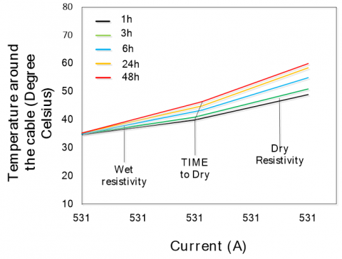
Figure 4 shows temperature distribution of the single-core cable system inside soil (0.6/1KV), which consists of three thermal circuits as a state study. These thermal circuits are directly buried in soil 1, soil 2 and soil 3, at depth of 0.8m, where distance between phases (from center to center) is 0.3m. Load current for every cable is 531 A. As well the temperature distribution at different types on the native soil are given separately in Figures 5-7. The graphs in all figures show two fairly linear parts of temperature around the cable versus load cycle with respect to time. The first part of the curve represents wet zone (or the soil thermal resistivity before it starts the dry case). The second part of the curve represents dry zone surrounding the cable. In other words, there are two slopes or zones. Dry zone is created around the cable, which represents the heat source under harsh environment and constant loading conditions. Wet zone begins from the end of dry zone. The cutout in the curves denotes the sorting between the wet resistivity and the dry resistivity (or dry zone and wet zone). Therefore, the soil thermal resistivity is proportional to the slope in every curve.
Interestingly enough, is that slope in every region shows an indication of the increment in resistivity for each type of the soil, which increases temperature around the cable in each case.
Simulations performed on different types of the soil showed that the ambient temperature (Ta) in summer season owns a main effect upon the cable temperature, and some generic notices can be described regarding the special situations studied in this paper. Under harsh environment and constant loading conditions, for every 8℃ increments in the ambient temperature, the cable temperature rise about 4℃.
Figure 4. Temperature distribution of the single-core cable system (three phases) directly buried in the soil 1 (0.6/1KV)
Figure 5. The drying curve for Soil 1 under severe environmental and unvarying loading circumstances for a period of between 1 and 48 hours
Figure 6. The drying curve for Soil 2 under adverse environmental circumstances, as well as the unvarying loading conditions for a period of between 1 and 48 hours
Figure 7. The drying curve of Soil 3 surrounding the cable under severe environmental and unvarying loading conditions for a period of between 1 to 48 hours
As a result, the air temperature in summer season leads to decrease the dissipated heat, which increases the critical temperature around the cable.
It is noticed that the unfavorable temperature (Tx) in the dry region and relationship between the dry and wet resistivity (or dry zone and wet zone) (V) rely on the components of the soil and the air temperature (seasonal changes).
Figure 8a. A heat flux density generated at the cables, which leads to the dry case under harsh environment and constant loading conditions
It is also noticed that the heat flux density generated under harsh environment and constant loading conditions is one of the most important factors, which determine the time required for the dry region as shown in Figure 8a and b. This is in reasonable and good agreement with studies [12, 29].
Remarkable conclusion in this study is that critical temperature not depends mainly on the heat flux from the cable as shown in Figure 8a and b. This may also be in agreement with Anderss [30], who proposed that the heat flux generated in the outer sheath of the cable is one of the important factors which determines the time required for soil change to unstable case. From Table 3, It can be seen that the critical temperature for each type of the soil under harsh environment and constant loading conditions are closer to 62℃ rather than the 50℃ that was commonly used by IEC [31].
Figure 8b. Heat gradient from heat source to soil under harsh environment conditions
Table 3. The critical temperature for different types of the native soil under harsh environment and constant loading conditions
|
Name of Soil |
Ta |
Tx |
$V=\frac{\rho\, d r y}{\rho\, w e t}$ |
Tx-Ta |
|
Soil 1 |
37 |
64 |
2.0312 |
27 |
|
Soil 2 |
35 |
60.3 |
1.671 |
25.3 |
|
Soil 3 |
34.5 |
61.7 |
2.041 |
27.2 |
In this paper, the derating factor is described as the ampacity (ampere capacity) of a cable computed upon the dry zone divided by the ampacity of the said cable while disregarding the dry zone as shown in Eq. (8).
$I=\frac{I \text { dry zone }}{\text { I without dry zone }}$ (8)
IEC 60287 standard offers a formula for calculating the ampacity of the dry zone. The employment of this formula calls for some information regarding certain parameters. These include that between critical and ambient temperatures, and that between the dry and wet zones (TX-Ta). Also required is the ratio of the resistivity of the dry zone to that of the wet zone (V). Objective of this work involves computations to determine the extent of these parameters Table 3.
The IEC guide 60287-1 provides an equation for computing the ampacity of underground cables with and without consideration to the influence of the dry zone phenomenon. The ampacity without consideration to the influence of the dry zone is computed as follows:
$\mathrm{I}=\left[\frac{\Delta \mathrm{T}-\mathrm{W}_{\mathrm{d}}\left\{0.5 \mathrm{~T}_1+\mathrm{n}\left(\mathrm{T}_2+\mathrm{T}_3+\mathrm{T}_4\right)\right\}}{\mathrm{R}_{\mathrm{ac}}\left\{\mathrm{T}_1+\mathrm{n}\left(1+\lambda_1\right) \mathrm{T}_2+\mathrm{n}\left(1+\lambda_1+\lambda_2\right)\left(\mathrm{T}_3+\mathrm{T}_4\right)\right\}}\quad\right]^{0.5}$ (9)
where, ∆T (Tc-Ta) Tc signifies the conductor temperature and Ta signifies the ambient temperature; n signifies the quantity of conductors; Wd signifies the dielectric loss of conductor lagging; Rac signifies AC resistance; T1 signifies the thermal resistance between conductor and sheath; T2 signifies the thermal resistance between bedding and sheath; T3 signifies the thermal resistance of the exterior serving of the cable; T4 signifies the thermal resistance between cable surface and ambient soil; λ1 signifies loss in the context of the metal sheath and; λ2 signifies losses related to protective coverings.
The adapted formula for computing the current-carrying capacity of the cable while taking into consideration the influence of the dry zone is exhibited below:
$\mathrm{I}=\left[\frac{\Delta \theta-\mathrm{W}_{\mathrm{d}}\left\{0.5 \mathrm{~T}_1+\mathrm{n}\left(\mathrm{T}_2+\mathrm{T}_3+\mathrm{VT}_4\right)\right\}+(\mathrm{V}-1) \Delta T_{\mathrm{x}}}{\mathrm{R}_{\mathrm{ac}}\left\{\mathrm{T}_1+\mathrm{n}\left(1+\lambda_1\right) \mathrm{T}_2+\mathrm{n}\left(1+\lambda_1+\lambda_2\right)\left(\mathrm{T}_3+\mathrm{VT}_4\right)\right\}}\,\,\quad\right]^{0.5}$ (10)
∆Tx (Tx-Ta) Tx symbolizes the critical temperature and Ta symbolizes the ambient temperature while; V symbolizes the ratio between dry resistivity and wet resistivity.
(Tx-Ta) Together with V are derived from Table 3 for dissimilar types of soil, while thermal resistivities are derived from Table 3. The computation of the derating factor for the present ratings of underground power cables was realized through the employment of the ETAP electrical engineering software. This computation involved the utilization of results acquired from tests conducted on a variety of soil types surrounding the cable. Table 4 Exhibits the results calculated through the program.
Table 4. The derating factor for three- phase cables (flat formation)
|
Type of Soil |
Soil 1 |
Soil 2 |
Soil 3 |
|
ρ wet |
1.27 |
1.29 |
1.21 |
|
ρ dry |
2.5 |
2.63 |
2.45 |
|
Temperature of dry zone |
64 |
60.3 |
61.7 |
|
600 volt |
|||
|
Ampacity without dry zone |
531 |
531 |
531 |
|
Ampacity with dry zone |
377 |
408 |
398 |
|
Derating factor |
0.71 |
0.75 |
0.76 |
It was observed that the derating factor at the dry zone ranges between 0.71 and 0.76, and that the dry zone for Soils 1, 2 and 3 developed at 64℃, 62℃ and 61.7℃ respectively according to the Eqs. (8) and (9). Other than the rating factors for a variety of soil types, Table 4 also provides a summing up of the calculated results for cable ampacity including and excluding the dry zone encircling the cable. From these results, it can be confirmed that Soils 2 and 3 come with a higher derating factor than Soil 1.
As displayed in this table, these soils are almost similar in terms of the disparity between critical and ambient temperatures, as well as the ratio of dry thermal resistivity to wet thermal resistivity. According to Table 3, although Soils 1, 2 and 3 have almost similar elements, the difference lies in the proportion of these parts. As Soil 1 registered the lowest derating factor, it follows that this soil has a higher dry thermal resistivity than wet thermal resistivity. This is displayed in Table 3. Its elevated dry thermal resistivity level is also due to the fact that it is made up almost entirely of sand without any trace of clay.
This paper concentrated on thermal behavior of the cable under extreme soil and environmental conditions. An overall method to deal with the relation between cable unfavorable working conditions and drating factors has been suggested. The approach utilized fundamental thermal and electrical concepts for determining the formation of the dry zone. Regarding to ordinary procedure defined through IEC-60287, in addition including harsh environmental conditions in hot countries. The governing equations were solved using finite element ANSYS Multiphysics and both soils and cables are included in the formation.
Results show that phenomenon the dry region in the soil begins at diverse temperature and diverse velocities at same the time period based on components of the soil. It also showed in this work is that the ambient air temperature (or harsh environment) has a major influence on cable temperature and the dry zone around the cable, as expected. In addition, remarkable conclusion in this work is that the critical temperature for the wet soils under harsh environment and constant loading conditions is closer to 62℃. As well as, the formation of dry zones around underground cables decreases the capacity of the cables by a factor of 0.71 to 0.76, which is defined in this paper as the derating factor; in addition, this factor depends basically on the type of soil.
[1] Hegyi, J., Klestoff, A.Y. (1988). Current-carrying capability for industrial underground cable installations. IEEE Transactions on Industry Applications, 24(1): 99-105. https://doi.org/10.1109/28.87258
[2] Hanna, M.A., Chikhani, A.Y., Salama, M.M.A. (1992). Thermal Analysis of Power Cables in Multi-layered Soil Part 1: Theory. In IEEE PES. Summer Meeting, 9(1): 572-578. https://doi.org/10.1109/61.252604
[3] Anders, G.J., Radhakrishna, H.S. (1988). Power cable thermal analysis with consideration of heat and moisture transfer in the soil. IEEE Transactions on Power Delivery, 3(4): 1280-1288. https://doi.org/10.1109/61.193921
[4] Anders, G.J., Napieralski, A.K.T., Zamojski, W. (1998). Calculation of the internal thermal resistance and ampacity of 3-core unscreened cables with fillers. IEEE Transactions on Power Delivery, 13(3): 699-705. https://doi.org/10.1109/61.686962
[5] De Leon, F., Anders, G.J. (2008). Effects of backfilling on cable ampacity analyzed with the finite element method. IEEE Transactions on Power Delivery, 23(2): 537-543. https://doi.org/10.1109/TPWRD.2008.917648
[6] Demoulias, C., Labridis, D.P., Dokopoulos, P.S., Gouramanis, K. (2006). Ampacity of low-voltage power cables under nonsinusoidal currents. IEEE Transactions on Power Delivery, 22(1): 584-594. https://doi.org/10.1109/TPWRD.2006.881445
[7] Garrido, C., Otero, A.F., Cidras, J. (2003). Theoretical model to calculate steady-state and transient ampacity and temperature in buried cables. IEEE Transactions on Power Delivery, 18(3): 667-678. https://doi.org/10.1109/TPWRD.2002.801429
[8] Yenchek, M.R., Cole, G.P. (1997). Thermal modelling of portable power cables. IEEE Transactions on Industry Applications, 33(1): 72-79. https://doi.org/10.1109/28.567080
[9] Anders, G.J., Napieralski, A., Kulesza, Z. (1999). Calculation of the internal thermal resistance and ampacity of 3-core screened cables with fillers. IEEE Transactions on Power Delivery, 14(3): 729-734. https://doi.org/10.1109/61.772307
[10] Schmidt, N.P. (1999). Comparison between IEEE and CIGRE ampacity standards. IEEE Transactions on Power Delivery, 14(4): 1555-1559. https://doi.org/10.1109/61.796253
[11] Anders, G.J., Chaaban, M., Bedard, N., Ganton, R.W.D. (1987). New approach to ampacity evaluation of cables in ducts using finite elemet technique. IEEE Transactions on Power Delivery, 2(4): 969-975. https://doi.org/10.1109/TPWRD.1987.4308208
[12] Donazzi, F., Occhini, E., Seppi, A. (1979). Soil thermal and hydrological characteristics in designing underground cables. In Proceedings of the Institution of Electrical Engineers, 126(6): 506-516. https://doi.org/10.1049/piee.1979.0119
[13] Calculations of the continuous current rating of cables (100% load factor). (1982). IEC Publication. 60287-1-3.
[14] Cigre, S.C. (1992). 21–Determination of a value of critical temperature rise for a cable backfill material. Electra ELT, 145(2): 15-30.
[15] Philip, J.R., De Vries, D.D. (1957). Moisture movement in porous materials under temperature gradients. Eos, Transactions American Geophysical Union, 38(2): 222-232. https://doi.org/10.1029/tr038i002p00222
[16] De Vries, D.A. (1975). Heat transfer in soils. In Heat and Mass Transfer in the Biosphere, edited by D. A. De H. Afgan, Scripta, Washington D.C., pp. 5-28.
[17] Gela, G., Dai, J.J. (1988). Calculation of thermal fields of underground cables using the boundary element method. IEEE Transactions on Power Delivery, 3(4). 1341-1347. https://doi.org/10.1109/61.193929
[18] Pichon, L., Razek, A. (1991). Thermal modeling of underground cables under transient conditions. Proceedings of JICABLE 91, pp. 475-482.
[19] Pichon, L., Razek, A. (1991). Echauffements Dans Les Ciibles Souterrains D'Energie - Calcul par une Technique Numtrique Mixte Eltments Finis-Elemknts de Frontibre. Revue GLnLrale de Thermique, 351: 171-176.
[20] Enescu, D., Colella, P., Russo, A., Porumb, R.F., Seritan, G.C. (2021). Concepts and methods to assess the dynamic thermal rating of underground power cables. Energies, 14(9): 2591. https://doi.org/10.3390/en14092591
[21] Alwan, S.H., Naife, R.M., Hadi, M.K. (2017). Derating Factors for underground power cables buried in non-uniform environmental conditions based on finite element method. International Journal of Electrical and Power Engineering, 11(1-6): 1-8. http://dx.doi.org/10.3923/ijepe.2017.1.8
[22] Bragatto, T., Cresta, M., Gatta, F.M., Geri, A., Maccioni, M., Paulucci, M. (2019). A 3-D nonlinear thermal circuit model of underground MV power cables and their joints. Electric Power Systems Research, 173: 112-121. https://doi.org/10.1016/j.epsr.2019.04.024
[23] Neher, J.H. (1949). The temperature rise of buried cables and pipes. Transactions of the American Institute of Electrical Engineers, 68(1): 9-21. https://doi.org/10.1109/T-AIEE.1949.5059897
[24] IEEE Std. 442-1981 IEEE Guide for Soil Thermal Resistivity Measurements.
[25] Mason, V.V., Krutz, M. (1952). Rapid method of thermal resistivity of soil. Transactions of the American Institute of Electrical Engineers, pp. 570-577. https://doi.org/10.1109/AIEEPAS.1952.4498511
[26] Martin, M.A., Bush, R.A., Black, W.Z., Hartley, J.G. (1981). Practical aspects of applying soil thermal stability measurements to the rating of underground power cables. IEEE Transactions on Power Apparatus and Systems, (9): 4236-4249. https://doi.org/10.1109/TPAS.1981.316975
[27] El-Kady, M.A. (1984). Calculation of the sensitivity of power cable ampacity to variations of design and environmental parameters. IEEE Transactions on Power Apparatus and Systems, (8): 2043-2050. https://doi.org/10.1109/TPAS.1984.318511
[28] Kellow, M.A. (1981). A numerical procedure for the calculation of the temperature rise and ampacity of underground cables. IEEE Transactions on Power Apparatus and Systems, (7): 3322-3330. https://doi.org/10.1109/TPAS.1981.316673
[29] Hartley, J.G., Black, W.Z. (1981). Transient simultaneous heat and mass transfer in moist, unsaturated soils. ASME Trans., 103: 376–382. https://doi.org/10.1115/1.3244469
[30] Anderss, G.J. (1998). Rating of Electric Power Cables. New York. IEEE Press/ McGraw-Hill.
[31] Freitas, D.S., Prata, A.T., de Lima, A.J. (1996). Thermal performance of underground power cables with constant and cyclic currents in presence of moisture migration in the surrounding soil. IEEE Transactions on Power Delivery, 11(3): 1159-1170. https://doi.org/10.1109/61.517467