Priyanga Subbiah![]() | Krishnaraj Nagappan*
| Krishnaraj Nagappan*![]()
© 2024 The authors. This article is published by IIETA and is licensed under the CC BY 4.0 license (http://creativecommons.org/licenses/by/4.0/).
OPEN ACCESS
Plant diseases significantly reduce the yield and the production of crops across the globe. Crop productivity, plant development and human access to food have all been hampered by the prevalence of plant diseases throughout the history. In general, leaves exhibit symptoms if the plant is affected by diseases. Therefore, it is essential to identify the type of infestation to reduce the destructiveness of the disease. This scenario allows one to replicate the spread of infectious diseases and the inability of farmers to recognize and remember them. One possible approach to tackle this issue is to utilise Deep Learning (DL) techniques in conjunction with Machine Learning (ML) approaches within the domain of Computer Vision (CV). The current research has introduced the APLDD-ESOSDL approach, which utilises deep learning to optimise the search for symbiotic organisms in order to automate the detection of plant leaf diseases. The objective of the proposed APLDD-ESOSDL approach is to enhance agricultural yields and reduce crop losses by offering farmers a visual depiction of disease symptoms. The goal of the APLDD-ESOSDL approach is to accurately classify the presence of leaf diseases. The APLDD-ESOSDL technique utilises the inception ResNet-v2 model as a feature extractor and the Stacked Long Short-Term Memory (SLSTM) model for classification. In addition, the hyperparameters of the SLSTM algorithm are adjusted using the Enhanced Symbiotic Organism Search (ESOS) approach. A comprehensive experiment was carried out utilising the reference data set to verify the effectiveness of the APLDD-ESOSDL approach. The APLDD-ESOSDL algorithm outperformed more advanced systems, achieving a maximum accuracy of 99.22%, precision of 98.52%, sensitivity of 98.06%, and specificity of 99.54% in experimental experiments employing six distinct cutting-edge approaches.
plant diseases; computer vision, agriculture, deep learning, parameter tuning, crop productivity, ESOS
Plant diseases adversely affect the agricultural productivity. Food insecurity may increase, if the plant diseases are not diagnosed promptly [1]. Earlier identification is vital for effective control and prevention of the plant diseases and they serve a crucial role in managing the agricultural productivity as well [2]. At present, plant disease detection remains a huge concern. Precise and prompt analysis of the plant diseases is critical for correct and sustainable agricultural production [3]. Certain plant diseases have invisible indications; in such cases, the advanced analyses techniques are used. However, most plant diseases start showing symptoms whereas skilled plant pathologists can sense the conditions and detect the disease by examining the affected plant leaves visually [4]. A pathologist should have good observation skills to find the characteristic symptoms in an accurate manner. However, the variations in the context of plant disease due to climatic changes, a large variety of plants and the faster spread of disease lead even skilled pathologists to misdiagnose some conditions [5].
In this background, the exploitation of intelligent and expert systems to automatically detect the plant disease precisely offers valuable contributions to agriculturists [6]. In addition, when these systems are presented as simple mobile apps, which non-expert farmers can easily use, it would be a great achievement and it helps the farmers to make decisions effectively. The recent developments in Artificial Intelligence (AI) technology have made a huge contribution to the advancement of automatic systems that can give precise and faster outcomes in disease diagnosis [7]. Recently, in the study of plant disease detection, Deep Learning (DL) technology has been further developed [8]. DL has expressed original image characteristics that contain numerous end-to-end features. Such characteristics make the DL technology obtain more attention in plant disease detection domain [9]. CNN, a type of DL method, is the preferable approach in disease detectio processes. It is well known for its potential in image processing and classification applications [10]. DL methods were first introduced in plant image detection based on leaf vein patterns.
1.1 Objective
The main goal behind early detection of plant diseases is to control it as it reduces the crop yields. Plant diseases have historically reduced the crop yields and endangered the food supply process. The aim of this research work is to develop a dynamic system that can accurately diagnose and classify the plant leaf diseases based on the symptoms observed in leaf pictures. This sort of identification is required for early illness detection and mitigation. The aim of the APLDD-ESOSDL is to classify the leaf diseases from plant pictures in an accurate manner. This classification is essential for decision-making in agriculture. The APLDD-ESOSDL method extracts the features using the Inception ResNet-v2 model. In general, image-based disease diagnosis requires feature extraction. The research uses Stacked Long Short-Term Memory (SLSTM) for disease classification. Sequential data analysis is SLSTM's forte. To improve the performance, the SLSTM’s hyperparameters are fine-tuned utilising the Enhanced Symbiotic Organism Search (ESOS). The study compares the performance of the APLDD-ESOSDL algorithm against the existing state-of-the-art systems to prove the former’s superiority. The method improves disease diagnosis accuracy and effectiveness.
Reddy et al. [11] proposed a new PDICNet method for identifying and diagnosing illnesses in plant leaves. The study employed the Modified Red Deer Optimizer Algorithm (MRDOA) as the optimal method for feature selection. The objective was to get conspicuous and ideal characteristics while decreasing the size of MRDOA. Furthermore, a DLCNN classifier method was utilised to enhance the accuracy of the classification. Abd Algani et al. [12] proposed a new deep learning method called Ant Colony Optimisation with Convolutional Neural Networks (ACO-CNN) to categorise and diagnose illnesses. This study evaluated the effectiveness of employing Ant Colony Optimisation (ACO) for the detection of illnesses in plant leaves. The CNN approach utilises many techniques to extract multiple pieces of information, such as the organisation of plant leaves, the geometric properties of texture, and the colour composition, from the provided photographs.
Shah et al. [13] developed a structure called Residual Teacher/Student (ResTS), which was utilised as a classification and visualisation method for diagnosing the plant diseases. ResTS is developed on the basis of CNN infrastructure with two classifiers (ResStudent and ResTeacher) and decoders. This structure trained both the classifiers from reciprocal mode and conveyed the representation between ResStudent and ResTeacher, in which the latter was utilised as a proxy. Hameed Al-bayati and Üstündağ [14] devised a Plant Disease Detection System (PDDS) structure using Deep Neural Network (DNN) that could diagnose apple plant leaf disease. For this study, Grasshopper Optimization Algorithm (GOA) was utilized for feature optimisation while Speeded Up Robust Feature (SURF) was used for the purpose of feature extraction. The classification parameters like Error, Precision, F-measure, Recall, and precision were determined and a comparative analysis was conducted to exhibit the effectiveness of the presented model. Albattah et al. [15] proposed a Custom CenterNet framework with DenseNet77 as a robust plant disease classification mechanism base network. As a primary step, the annotations were presented to acquire the RoI. In the secondary step, an improved CenterNet was projected while DenseNet77 was developed for abstracting deep vital points. In order to find and classify the plant diseases, the 1-stage detector CenterNet was adopted in this study.
Alirezazadeh et al. [16] modelled the CBAM (Convolutional Block Attention Module) for enhancing the classification outcomes with CNN, a lightweight attention module embedded as some CNN structure with negligible overhead. Some of the renowned CNN methods (i.e., ResNet50, EfficientNetB0, VGG19, MobileNetV2, and InceptionV3) were implemented for executing the TL for classifying plant diseases and then fine-tuning using the plant disease database. In literature [17], a DCNN method was developed for image-related plant leaf disease detection utilising hyperparameter optimization and data augmentation techniques.
Chakraborty et al. [18] presented an approach for performing multilayer picture thresholding by employing the Symbiotic Organisms Search (SOS) algorithm. The SOS algorithm demonstrated a superior performance than the four contemporary meta-heuristic algorithms. The SOS algorithm effectively achieved an optimal balance between intensity and diversification. This study introduced a novel approach for doing multilevel image thresholding. The concept of symbiotic relationships among the organisms was employed to enhance the objective functions. Chakraborty et al. [19] introduced a new optimisation technique called Chaotic Symbiotic Organisms Search (CSOS) for multilevel picture segmentation. The aim of the proposed method was to enhance the performance of the traditional Symbiotic Organisms Search (SOS) algorithm in image processing [20]. The effectiveness of the CSOS algorithm was demonstrated in combination with Masi's entropy. The CSOS method had a broad range of flexibility, particularly in high-dimensional optimization problems.
2.1 Limitations
The reference dataset studies exhibited the accuracy, precision, sensitivity, and specificity of the proposed method. However, real-world illumination, leaf changes, and ambient circumstances may cause the proposed model to malfunction. Inception ResNet-v2 and SLSTM models get affected by quality and quantity of the training data. If the training dataset does not represent all types of scenarios, the algorithm may struggle to identify the plant diseases in diverse species and conditions. Plant diseases tend to exhibit different types of symptoms. This approach may misdiagnose rare or early diseases. The training dataset may be imbalanced, when some disease classes have only a few examples. The model may classify the underrepresented diseases poorly.
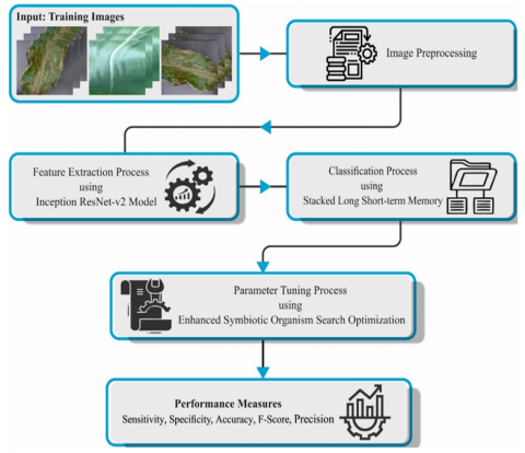
In the current study, a novel APLDD-ESOSDL technique has been presented for accurate detection and classification of plant leaf diseases. The aim of the given technique is to categorize the presence of leaf diseases properly. The proposed technique encompasses several stages of operations. The SLSTMs are ideal for sequential data problems like time series and image sequences. Plant leaf disease diagnosis involves a series of changes in leaf symptoms. The SLSTMs can capture temporal relationships, which helps in disease detection process. LSTMs and other deep learning models excel at image classification. The capacity to automatically learn and extract the features from image data can help in identifying tiny leaf disease changes. Traditional machine learning methods may struggle to capture complicated leaf disease patterns and linkages. As deep learning models, the SLSTMs can represent complex data relationships. ESOS is a metaheuristic optimisation technique that functions on the basis of natural symbioses. This technique is specialized in efficient exploration of the parameter spaces and the detection of optimal or near-optimal solutions. When used for hyperparameter adjustment, ESOS can improve the parameters of the model. Preventing overfitting in deep learning models requires hyperparameter adjustment. ESOS helps in identifying the hyperparameters that balance the model’s complexity with generalisation. The customization of ESOS towards specific optimisation aims makes it suitable for plant leaf disease diagnostics. For noise reduction and image edge preservation, bilateral filtering is an efficient option. BF can improve the plant leaf picture data for analysis, even with noise or flaws. BF enhances the essential visual elements and hides the unimportant ones. This can assist the model focus on disease-related features and reduce unnecessary image artefacts. Pre-processing methods like BF can improve the model’s performance by cleaning and informing the input data. These methods are chosen because they can handle sequential data, optimise the model’s performance, and preprocess the images for plant leaf disease identification. The researchers must provide detailed arguments in their study to confirm these design decisions and establish its efficacy compared to other methodologies. Figure 1 illustrates the workflow of the APLDD-ESOSDL approach.
Figure 1. Workflow of the APLDD-ESOSDL approach
Many task-specific factors have been studied for Inception ResNet-v2 model based feature extraction. This application benefits from unique architecture and computer vision. The essential reasons to use the inception ResNet-v2 model are listed below.
1. Beginning deep residual link: Architecture Inception from GoogLeNet helps in ResNet-v2 model’s reuse connections. The deep hybrid model captures both low- as well as high-level traits. This depth is needed to extract the correct patterns and structures from complex multi-scale medical images.
2. Multi-scale feature extraction: Inception ResNet-v2 model have varied convolutional filter sizes. The multi-scale approach accounts for medical imaging variability by collecting the characteristics at multiple granularities. The model should have adaptability since it should work with healthcare data images of various resolutions, orientations, and textures.
3. Inception in computer vision: ResNet-v2 governs the classification process. Classification, object recognition, and segmentation are handled for varied image datasets. The proposed model extracts task-relevant information and executes differentiation.
4. Transfer learning inception: Transfers the learning outcomes from the ImagesNet ResNet-v2. The training data and representations are used with pre-trained models. When updated with the medical imaging dataset, the model responds quickly and saves data from processing.
5. Inception: efficiency and scalability: Model complexity and computational efficiency are balanced by ResNet-v2 model while the computationally-light healthcare software benefits from the deep design of the model. Scalability lets us to add features or alter the models.
3.1 Image pre-processing
To improve the quality of plant leaf disease images, Bilateral Filtering (BF) technique is used. BF is a noise removal technique inspired by Gaussian filtering (GF) technique [19]. But, by effectually preserving the denoising ability of GF, it efficiently reduces the additive noise without ending the specifics and edges of the images. The edge data of the images are maintained though the impulse noise cannot be separated.
3.2 Feature extraction process
For effectual extraction of the features, the Inception ResNet-v2 model is used. Transfer Learning (TL) is a branch of ML that proposes data transmission in a source model for objective function by utilising the correlations in parts, models, or outcomes [20]. For the TL model, the Inception‐Resnet‐V2 structure with pre-training weighted is utilised. The network model can learn rich element representations for different images. Different sizes of convolution filters and residual networks can be combined in the Inception‐Resnet block. The stimulus to choose this structure was based on the experimental outcomes and comparison study with other DL approaches. As the model is considered to be used in edge platform, other resource‐extensive, bulky methods cannot be selected.
The residual networks offer model shortcuts, thus permitting this structure to achieve even more superior outcomes. It is a hybrid of residual and inception blocks, which enhances the efficiency. In order to improve the efficiency of the trained model, the Inception accomplishes optimum utilisation of the computational resources and removes further features with similar computation counts. The resultant of the previous layer is integrated with the network after which the computation of the 5×5 convolutional kernel gets large. The 1×1 convolutional is utilised in the Inception element for two reasons: the primary reason is to overlap more convolutions on receptive domains of similar scale to derive rich features in the constellation diagram. The second reason is to reduce the computational cost and measurement. The 1×1 convolutional layer of the network that derives before 3×3 and 5×5 convolutional layers is utilized for reducing the dimensionality issues. This method is determined to strike a right balance between overfitting and underfitting. The dense layers utilize the ReLU activation function, which is mathematically determined utilizing the subsequent formula:
$R(Z)=\max (0, Z)$ (1)
The FC layer is exchanged with global average pooling layer excluding the inception model’s elements. It is complete to reduce the variable counts. Batch Normalization (BN) also forms a part of the network procedure. The BN layer creates the entire mini‐batch constellation maps that are similar to it moving forward to NN layer, thus avoiding the gradients from disappearing problem.
It is a group of constellations that assists the trained ground to provide some of the constellation. The BP technique also computes the Jacobians. These are easily partial derivations of norms for the variables $a$ and $\chi$.
$\frac{\sigma \operatorname{Norm}(a, \chi)}{\partial a}$ and $\frac{\sigma \operatorname{Norm}(a, \chi)}{\partial \chi}$ (2)
In this network, Adam optimization algorithm is utilized for maximizing the network parameter and minimizing the loss. This model is highly effective if the functioning of the model has huge issues with several data or parameters. It is effectual and needs minimal memory.
$\theta_x:=\theta_{x-1}-\alpha \cdot \frac{\widehat{m}_x}{\sqrt{v} x+\varepsilon}$ (3)
At this point, $\alpha \in R$ and $\theta, \widehat{m}_t, \hat{v}_t, e \in R^n$ for some $n$.
To this day, dropout's regularisation feature is useful for avoiding overfitting issues. In the majority of instances, the dropout may be seen as a sign that a neuron of NN is disabled during training with a certain probability p. The following formula demonstrates the following method for calculating the dropout for the probability $p_i(1 \leq i \leq t)$.
$E_R=\frac{1}{2}\left(x-\sum_{i=1}^t p_i w_i I_i\right)^2+\sum_{i=1}^t p_i\left(1-p_i\right) w_i^2 I_i^2 a$ (4)
3.3 Plant leaf disease classification model
In order to accurately identify and categorise diseases affecting plant leaf tissue, the SLSTM model is employed. The SLSTM model is an LSTM stack, which consists of many stacked layers. Hence, the subsequent layer takes its input from the previous layer's LSTM output [21]. The LSTM model makes use of three gates. Each of the three types of gates input, output, and forget has a single cell state. The LSTM receives as inputs in each time-step t the hidden state $h_{t-1}$ and the cell state $c_{t-1}$, which were created in the time-step before t-1. The input t-1, is obtained in the following way at the current time t:
$h_t, c_t=f_{L S T M}\left(u_t, h_{t-1}, c_{t-1}\right)$ (5)
An explanation of the internal structure of the LSTM model's memory cells and gates is provided below.
$i_t=\sigma\left(W_i u_t+R_i h_{t-1}+b_i\right)$ (6)
$f_t=\sigma\left(W_f u_t+R_f h_{t-1}+b_f\right)$ (7)
$o_t=\sigma\left(W_o u_t+R_o h_{t-1}+b_o\right)$ (8)
$z_t=\tanh \left(W_z u_t+R_z h_{t-1}+b_z\right)$ (9)
$c_t=i_t \odot+f_t \odot c_{t-1}$ (10)
$h_t=0_t \odot \tanh \left(c_t\right)$ (11)
A bias vector is represented by the letter b, the input weight matrix that was learnt during training by the letter W, and the recurrent weight matrix by the letter R in this context. Furthermore, the sigmoid function, denoted by the equation $(x)=1 / 1+\exp (x)$, is also represented by the symbol σ. On top of that, it compresses the input to a range of values between zero and one, thanks to its squashing effect. To avoid a drastic rise in value over time, the hyperbolic tangent function Tanh generates values between -1 and 1, thereby limiting the range of possible values. Finding the values of these two functions requires a computation that takes each component into account. The symbol $i_t$ represents the input gate, $o_t$ represents the output gate, and $f_t$ represents the forget gate. The output of the sigmoid function is used to calculate the linear projections. These projections are then added to the linear projections of $u_t$ and $h_{t-1}$. The forget, input, and output gates are utilised to modulate the cell value of the prior state $c_{t-1}$, the input conversion $z_t$, and the component-wise multiplication output $\odot$, respectively. By utilising a three-layer stacked LSTM architecture, the output of the third layer is directly fed as input to the second layer, while the output of the first layer serves as the input for the second layer. In order to obtain the concealed states and initial cell, we compute the mean of the collections of the vector p. For the first LSTM layer, they are $c_0^1$ and $h_0^1$. For the second LSTM layer, they are $c_0^2$ and $h_0^2$. Finally, for the third LSTM layer, they are $c_0^3$ and $h_0^3$. Two different Multi-Layer Perceptrons (MLP) are used to process these evaluations; they are represented as $f_{i n i t_{-C}}^i$ and $f_{i n i t_{-} h}^i, i$ respectively, where $i=1,2,3$:
$h_0^i=f_{i n i t_{-} h}^i\left(\frac{1}{L} \sum_i^L a_i\right)$ (12)
$c_0^i=f_{i n i t_{-C}}^i\left(\frac{1}{L} \sum_i^L a_i\right)$ (13)
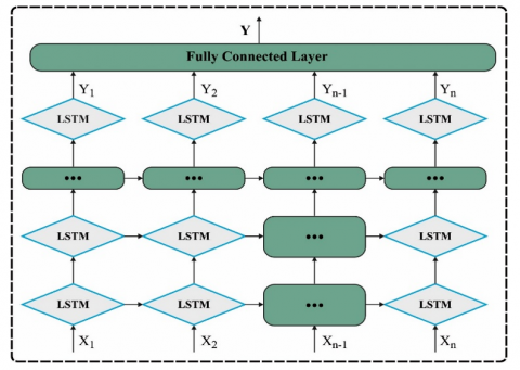
The annotation vectors $a_i$ where i ranges from 1 to L, represent the characteristics associated with certain sub-regions of the picture. In addition, an initial layer of LSTM uses a multi-layer LSTM stack. Figure 2 depicts the structure of the SLSTM technology.
3.4 Parameter tuning process
For the optimal selection of the hyperparameters related to the SLSTM model, the ESOS algorithm is used. SOS creates a population initialization of the organisms in which all the organisms are created randomly in a predetermined search space [22]. During the iteration or generation process, this algorithm exploits parasitism, mutualism, and commensalism to find the optimum global solution.
Figure 2. Structure of SLSTM
3.4.1 Mutualism phase
The term "mutualism" is used to describe symbiotic partnerships where two species work together and both parties benefit from the association. From the population, two distinct organisms, $X_i^g$ and $X_{R_1}^g$, are chosen at random. Here we have the tangible illustration. Two new species are born from the mating of the two animals, as seen below.
$X_{\text {inew }}^g=X_i^g+\operatorname{rand}[0,1]\left(X_{\text {best }}^g-B P 1 * M v\right)$ (14)
$X_{R_1 \text { new }}^g=X_{R_1}^g+\operatorname{rand}[0,1]\left(X_{\text {bes }}^g-B F 2 * M v\right)$ (15)
$M v=\frac{X_i^g+X_{R_1}^g}{2}$ (16)
In this context, $X_{\text {best }}^g$ represents the most superior individual organism in the current population. The term rand [0,1] refers to a randomly generated value within the range of 0 to 1. BF1 and BF2 are variables that represent the benefit factors of all organisms. These factors are randomly generated as either 1 or 2, depending on whether the benefits during the interaction are full or partial. Afterwards, $X_{\text {inew }}^g$ and $X_{R_1 \text { new }}^g$ are calculated using the primary function. These values are then compared against $X_i^g$, and $X_{R_1}^g$ in order to identify the most optimal organisms in each pair.
3.4.2 Parasitism phase
One kind of symbiotic interaction occurs when one organism gains an advantage over another, while the other organism has negative consequences. The present population or environment is used to randomly choose $X_i^g$ and $X_{R_1}^g$ to start. Furthermore, $X_{\text {parasite }}^g$ stands for an organism that is present in the population or environment in the form of a copy. The subsequent creation of a parasitic organism is the responsibility of $X_{\text {parasite }}^g$. The host organism for the parasite is represented by $X_{R_1}^g$. The $X_{\text {parasite }}^g$. modifies some of its components at random so that it can affect the host.
$X_{\text {parasite }}^g=L+\operatorname{rand}[0,1](U-L)$ (17)
If $X_{\text {parasite }}^g$ has a higher objective function value than the host organism $\left(X_{R_1}^g\right)$, then $X_{\text {parasite }}^g$ can replace the host organism in the present environment. Algorithm 1 depicts the common architecture of the SOS algorithm.
In the ESOS algorithm, the chaotic optimizer technique is utilized for initializing the population. The chaotic logistic mapping system decides the initialized population. Chaotic modification support the prevention of local minima by presenting arbitrary perturbation as the search model. This perturbation supports the model for exploring the searching space regions, which it could not be searched. Chaos is established as the searching procedure to make this technique highly possible to determine the global minima and less possibly to get stuck in local minima. The mathematical equation of the chaotic logistic mapping is as follows:
$y(1)=\operatorname{rand}, y(i+1)=r y(i)(1-y(i))$ (18)
where, rand denotes the random integer that lies in the range of 0 and $1, r$ signifies the specific variable of the logistic map with a value of 4. Next, the population is initialized using the subsequent formula, assuming that $(L B)$ lower bound and $(U B)$ upper bound of the optimizer parameter.
$P(i)=y(i) \cdot(U B-L B)+L B$ (19)
In Eq. (19), the counter $i$ counts from 1 to $N$ and $P$ signifies the place.
|
Algorithm 1: Pseudocode of the SOS algorithm |
|
START Specify the following parameters: population size (n), objective function $(X)$, limits on search variables $(L B, U B)$, number of search variables $(\mathrm{m}$ ), and either the maximum number of generations $g_{\text {max }}$ or the maximum number of function evaluations ( ( $F E_{\max }$) as the ending criteria. Here, $f(X)$ represents the objective function, and $X$ represents the search vector. Initiating random population, Compute the fitness of populations, $F E=0$, FOR $g=1$ to $g_{\max }$ DO; Sort the population in ascending order of $f\left(X_i\right)$ values, Find the better solution ( $\left.X_{\text {best}}\right)$ for the populations. $\text { FOR } i=1 \text { to } n \text { Do }$ $\begin{aligned} & B F 1=1+\operatorname{round}[\operatorname{rand}(0,1)] \\ & B F 2=1+\operatorname{round}[\operatorname{rand}(0,1)]\end{aligned}$ $M V=\left(X_i+X_k\right) / 2$ $\begin{gathered}X_i^{\prime}=X_i+\operatorname{rand}\left(0_J 1\right)+\left(X_{\text {best }}-M V * B F 1\right) \\ X_k^{\prime}=X_k+\operatorname{rand}(0,1)+\left(X_{\text {best }}-M V * B F 2\right) \\ F E=F E+2\end{gathered}$ IF $f\left(X_i^{\prime}\right)<f\left(X_i\right)$ THEN $\mid X_i=X_i^{\prime}$ END IF IF $f\left(X_k^{\prime}\right)<f\left(X_k\right)$ THEN $\mid X_k=X_k^{\prime}$ END IF $\begin{aligned} IF $f\left(X_i^{\prime}\right)<f\left(X_i\right)$ THEN $\mid X_i=X_i^{\prime}$ END IF Choose Parasite Vector $F E=F E+1$ IF $f$ (Parasite Vector) $<f\left(X_k\right)$ THEN $\mid X_k=$ Parasite Vector END IF IF $F E \geq F E_{\max }$ THEN | Break optimization loop END IF END FOR Report best solution END |
Fitness Function is a vital feature in the ESOS algorithm. An encoder result can be employed to assess the aptitude of the candidate result. At this point, accuracy is the major factor exploited to scheme a fitness function.
Fitness $=\max (P)$ (20)
$P=\frac{T P}{T P+F P}$ (21)
This section assesses the effectiveness of the APLDD-ESOSDL system in identifying plant leaf diseases. The evaluation is based on the plant disease dataset obtained from the Kaggle repository [23]. The dataset comprises 3,503 samples that have been categorised into four categories, as seen in Table 1.
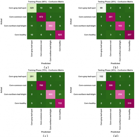
In Figure 3, the confusion matrices generated by the APLDD-ESOSDL technique for plant leaf disease detection and classification are portrayed. The results represent that the APLDD-ESOSDL technique properly categorized different types of plant leaf diseases.
Table 1. Details of the database
|
Class |
No. of Samples |
|
Corn gray spot |
466 |
|
Corn rust |
1084 |
|
Corn northern blight |
896 |
|
Corn healthy |
1057 |
|
Total Number of Samples |
3503 |
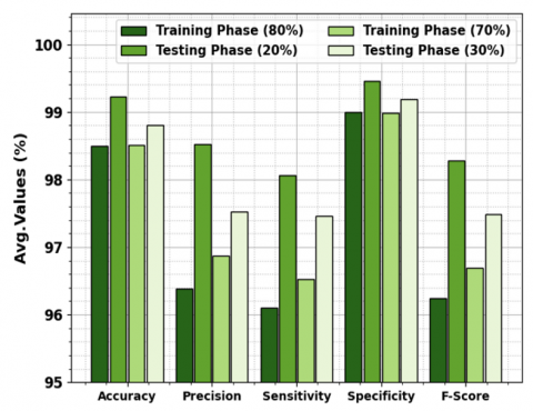
The APLDD-ESOSDL approach clearly presents a complete result of plant leaf disease detection in Table 2 and Figure 4. The experimental results indicate that the APLDD-ESOSDL approach achieved effective outcomes in all four categories. The APLDD-ESOSDL approach produced an average accuracy of 98.50%, precision of 96.39%, sensitivity of 96.11%, specificity of 99%, and F-score of 96.25% with 80% of TRP. Similarly, while using 20% of TSP, the APLDD-ESOSDL method achieved average accuracy, precision, sensitivity, specificity, and F-score values of 99.22%, 98.52%, 98.06%, 99.46%, and 98.28% respectively. The APLDD-ESOSDL approach achieved an average accuracy of 98.51%, precision of 96.87%, sensitivity of 96.52%, specificity of 98.98%, and F-score of 96.69% with 70% of TRP. The APLDD-ESOSDL system achieved an average accuracy of 98.81%, precision of 97.52%, sensitivity of 97.46%, specificity of 99.19%, and F-score of 97.49% with a TSP of 30%.
Figure 3. Confusion matrices of APLDD-ESOSDL approach (a-b) 80:20 of TRP/TSP and (c-d) 70:30 of TRP/TSP
Table 2. Plant leaf disease detection outcomes of the APLDD-ESOSDL approach under distinct measures
|
Class |
Accurcy |
Precision |
Sensitivity |
Specificity |
F-score |
|
Training Phase (80%) |
|||||
|
Corn gray spot |
97.79 |
92.58 |
90.78 |
98.83 |
91.67 |
|
Corn rust |
98.87 |
97.77 |
98.77 |
99.11 |
98.26 |
|
Corn northern blight |
98.58 |
97.50 |
97.09 |
99.09 |
97.30 |
|
Corn healthy |
98.37 |
97.30 |
97.42 |
98.78 |
97.36 |
|
Average |
98.40 |
96.29 |
96.01 |
99.10 |
96.15 |
|
Testing Phase (20%) |
|||||
|
Corn gray spot |
99.04 |
99.10 |
95.09 |
99.73 |
97.16 |
|
Corn rust |
99.04 |
97.47 |
99.40 |
99.10 |
98.43 |
|
Corn northern blight |
99.47 |
98.82 |
99.36 |
99.51 |
99.09 |
|
Corn healthy |
99.00 |
98.47 |
98.00 |
99.29 |
98.24 |
|
Average |
99.12 |
98.42 |
98.16 |
99.36 |
98.18 |
|
Training Phase (70%) |
|||||
|
Corn gray spot |
98.68 |
96.14 |
94.07 |
99.34 |
95.00 |
|
Corn rust |
99.08 |
98.36 |
98.87 |
99.18 |
98.61 |
|
Corn northern blight |
98.18 |
97.19 |
95.29 |
99.11 |
96.13 |
|
Corn healthy |
98.10 |
95.78 |
97.47 |
98.09 |
96.62 |
|
Average |
98.41 |
96.77 |
96.42 |
98.88 |
96.59 |
|
Testing Phase (30%) |
|||||
|
Corn gray spot |
99.15 |
96.52 |
96.72 |
99.64 |
96.72 |
|
Corn rust |
99.14 |
98.79 |
99.25 |
99.09 |
98.62 |
|
Corn northern blight |
98.28 |
97.61 |
95.78 |
99.13 |
96.69 |
|
Corn healthy |
98.47 |
97.38 |
97.69 |
98.81 |
97.54 |
|
Average |
98.71 |
97.42 |
97.36 |
99.09 |
97.39 |
Figure 4. Average outcomes of the APLDD-ESOSDL approach under distinct measures
Figure 5. Accuracy curve of the APLDD-ESOSDL approach
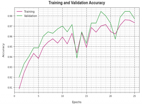
Figure 5 assesses the level of accuracy achieved by the proposed approach in both the training and validation models using the test database. The results suggest that the proposed approach demonstrated superior accuracy as the number of epochs grew. Moreover, the observation that the greatest validation accuracy surpasses the training accuracy suggests that the proposed algorithm successfully acquired knowledge from the test database.
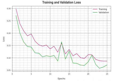
Figure 6 presents the results of the loss study for the proposed system during the training and validation phases, primarily focusing on the test database. The outcome indicates that the proposed approach yielded comparable values for both the training and validation loss. The proposed approach effectively showed its ability to learn from the test database.
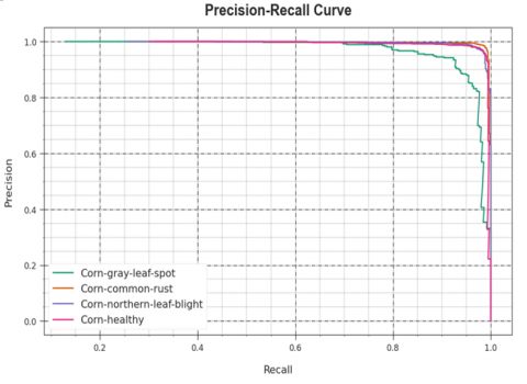
Figure 7 displays a comprehensive Precision-Recall (PR) curve of the APLDD-ESOSDL technique using the test database. The outcome indicates the effectiveness of the APLDD-ESOSDL system based on the highest PR values. Moreover, it is evident that the APLDD-ESOSDL method may achieve higher PR values for all the classes.
Figure 6. Loss curve of the APLDD-ESOSDL approach
Figure 7. PR curve of the APLDD-ESOSDL approach
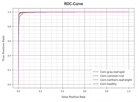
Figure 8 displays the results of the ROC analysis produced by the APLDD-ESOSDL technique on the test database. The data suggests that the APLDD-ESOSDL system attained the highest ROC values. Furthermore, it is evident that the APLDD-ESOSDL technique may achieve higher ROC values for all the classes.
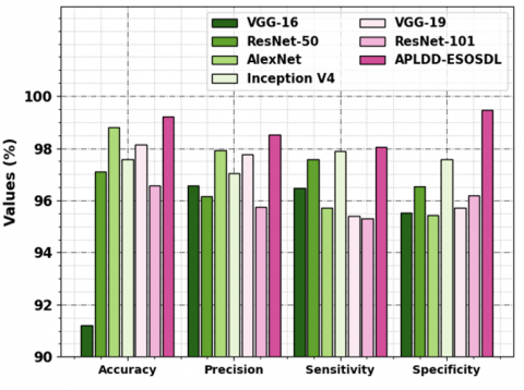
The findings of the full comparison analysis of the APLDD-ESOSDL approach and other state-of-the-art techniques are presented in Table 3 and Figure 9 [24]. The findings indicate that the VGG-16 model performed the poorest, while the ResNet-50, Inception V4, and ResNet-101 models produced somewhat better results. Simultaneously, the AlexNet and VGG-19 models achieved significant performance. The APLDD-ESOSDL approach shown exceptional performance, with a maximum accuracy of 99.22%, precision of 98.52%, sensitivity of 98.06%, and specificity of 99.46%. The findings unequivocally demonstrated the superior performance of the APLDD-ESOSDL approach compared to other models.
Figure 8. ROC curve of the APLDD-ESOSDL approach
Figure 9. Comparative outcome of APLDD-ESOSDL approach with recent systems
Table 3. Comparative analysis outcomes of the APLDD-ESOSDL approach with recent systems
|
Model |
Accuracy |
Precision |
Sensitivity |
Specificity |
|
VGG-16 |
91.20 |
96.58 |
96.48 |
95.54 |
|
ResNet-50 |
97.10 |
96.15 |
97.57 |
96.52 |
|
AlexNet |
98.80 |
97.93 |
95.73 |
95.44 |
|
Inception V4 |
97.59 |
97.03 |
97.89 |
97.56 |
|
VGG-19 |
98.13 |
97.77 |
95.39 |
95.73 |
|
ResNet-101 |
96.56 |
95.76 |
95.3 |
96.19 |
|
APLDD-ESOSDL |
99.22 |
98.52 |
98.06 |
99.46 |
In this article, have introduced a new approach called APLDD-ESOSDL for precise identification and categorization of plant leaf diseases. The objective of the proposed is to provide farmers with visual descriptions of plant leaf pictures in order to mitigate the spread of disease, hence enhancing agricultural yield and minimising crop losses. The proposed approach accurately classifies the occurrence of leaf diseases. The proposed approach consists of many steps, including feature extraction based on Inception ResNet-v2, classification using SLSTM, and hyperparameter tuning using ESOS. In order to identify the superior characteristics of the proposed technique, a widespread experimental analysis was conducted using the benchmark database. The experimental outcomes demonstrated the improved results of the proposed system in comparison with existing systems in terms of various performance measures. The current research outcomes improve precision in agricultural practices. The capacity to precisely identify and target the sick plants improves resource allocation and tailored therapy. This aids the worldwide sustainable agriculture movement to address the challenges posed upon food security and the environment. The current study is linked to these scientific goals and its real-world applications to stress its potential to increase plant leaf disease detection and solve important farmer and agricultural sector concerns. In the future, the classification performance of the APLDD-ESOSDL technique can be improved by multi-modal fusion approach. Multi-modal fusion may improve the classification accuracy, robustness, and generalisation. Integrating and fusing the data from several sources can help in building more powerful models for difficult categorization problems.
[1] Hernández, S., López, J.L. (2020). Uncertainty quantification for plant disease detection using Bayesian deep learning. Applied Soft Computing, 96: 106597. https://doi.org/10.1016/j.asoc.2020.106597
[2] Arsenovic, M., Karanovic, M., Sladojevic, S., Anderla, A., Stefanovic, D. (2019). Solving current limitations of deep learning based approaches for plant disease detection. Symmetry, 11(7): 939. https://doi.org/10.3390/sym11070939
[3] Hong, H., Lin, J., Huang, F. (2020). Tomato disease detection and classification by deep learning. In 2020 International Conference on Big Data, Artificial Intelligence and Internet of Things Engineering (ICBAIE), Fuzhou, China, pp. 25-29. https://doi.org/10.1109/ICBAIE49996.2020.00012
[4] Jayaprakash, K., Balamurugan, S.P. (2023). Artificial rabbit optimization with improved deep learning model for plant disease classification. In 2023 5th International Conference on Smart Systems and Inventive Technology (ICSSIT), Tirunelveli, India, pp. 1109-1114. https://doi.org/10.1109/ICSSIT55814.2023.10061156
[5] Jasim, M.A., Al-Tuwaijari, J.M. (2020). Plant leaf diseases detection and classification using image processing and deep learning techniques. In 2020 International Conference on Computer Science and Software Engineering (CSASE), Duhok, Iraq, pp. 259-265. https://doi.org/10.1109/CSASE48920.2020.9142097
[6] Moupojou, E., Tagne, A., Retraint, F., Tadonkemwa, A., Wilfried, D., Tapamo, H., Nkenlifack, M. (2023). FieldPlant: A dataset of field plant images for plant disease detection and classification with deep learning. IEEE Access, 11: 35398-35410. https://doi.org/10.1109/ACCESS.2023.3263042
[7] Goyal, L., Sharma, C.M., Singh, A., Singh, P.K. (2021). Leaf and spike wheat disease detection & classification using an improved deep convolutional architecture. Informatics in Medicine Unlocked, 25: 100642. https://doi.org/10.1016/j.imu.2021.100642
[8] Marzougui, F., Elleuch, M., Kherallah, M. (2020). A deep CNN approach for plant disease detection. In 2020 21st International Arab Conference on Information Technology (ACIT), Giza, Egypt, pp. 1-6. https://doi.org/10.1109/ACIT50332.2020.9300072
[9] Mzoughi, O., Yahiaoui, I. (2023). Deep learning-based segmentation for disease identification. Ecological Informatics, 75: 102000. https://doi.org/10.1016/j.ecoinf.2023.102000
[10] Darwish, A., Ezzat, D., Hassanien, A.E. (2020). An optimized model based on convolutional neural networks and orthogonal learning particle swarm optimization algorithm for plant diseases diagnosis. Swarm and Evolutionary Computation, 52: 100616. https://doi.org/10.1016/j.swevo.2019.100616
[11] Reddy, S.R., Varma, G.S., Davuluri, R.L. (2023). Resnet-based modified red deer optimization with DLCNN classifier for plant disease identification and classification. Computers and Electrical Engineering, 105: 108492. https://doi.org/10.1016/j.compeleceng.2022.108492
[12] Abd Algani, Y.M., Caro, O.J.M., Bravo, L.M.R., Kaur, C., Al Ansari, M.S., Bala, B.K. (2023). Leaf disease identification and classification using optimized deep learning. Measurement: Sensors, 25: 100643. https://doi.org/10.1016/j.measen.2022.100643
[13] Shah, D., Trivedi, V., Sheth, V., Shah, A., Chauhan, U. (2022). ResTS: Residual deep interpretable architecture for plant disease detection. Information Processing in Agriculture, 9(2): 212-223. https://doi.org/10.1016/j.inpa.2021.06.001
[14] Hameed Al-bayati, J.S., Üstündağ, B.B. (2020). Evolutionary feature optimization for plant leaf disease detection by deep neural networks. International Journal of Computational Intelligence Systems, 13(1): 12-23. https://doi.org/10.2991/ijcis.d.200108.001
[15] Albattah, W., Nawaz, M., Javed, A., Masood, M., Albahli, S. (2022). A novel deep learning method for detection and classification of plant diseases. Complex & Intelligent Systems, 8: 507-524. https://doi.org/10.1007/s40747-021-00536-1
[16] Alirezazadeh, P., Schirrmann, M., Stolzenburg, F. (2023). Improving deep learning-based plant disease classification with attention mechanism. Gesunde Pflanzen, 75(1): 49-59. https://doi.org/10.1007/s10343-022-00796-y
[17] Pandian, J. A., Kanchanadevi, K., Kumar, V.D., Jasińska, E., Goňo, R., Leonowicz, Z., Jasiński, M. (2022). A five convolutional layer deep convolutional neural network for plant leaf disease detection. Electronics, 11(8): 1266. https://doi.org/10.3390/electronics11081266
[18] Chakraborty, F., Roy, P.K., Nandi, D. (2020). Symbiotic organisms search optimization for multilevel image thresholding. International Journal of Swarm Intelligence Research (IJSIR), 11(2): 31-61. https://doi.org/10.4018/IJSIR.2020040103
[19] Chakraborty, F., Roy, P.K., Nandi, D. (2021). A novel chaotic symbiotic organisms search optimization in multilevel image segmentation. Soft Computing, 25(10): 6973-6998. https://doi.org/10.1007/s00500-021-05611-w
[20] Pandey, A., Jain, K. (2022). A robust deep attention dense convolutional neural network for plant leaf disease identification and classification from smart phone captured real world images. Ecological Informatics, 70: 101725. https://doi.org/10.1016/j.ecoinf.2022.101725
[21] Katiyar, S., Borgohain, S.K. (2021). Image captioning using deep stacked LSTMs, contextual word embeddings and data augmentation. arXiv preprint arXiv:2102.11237. https://doi.org/10.48550/arXiv.2102.11237
[22] Ganesh, N., Shankar, R., Kalita, K., Jangir, P., Oliva, D., Pérez-Cisneros, M. (2023). A novel decomposition-based multi-objective symbiotic organism search optimization algorithm. Mathematics, 11(8): 1898. https://doi.org/10.3390/math11081898
[23] PlantVillage Dataset. https://www.kaggle.com/datasets/emmarex/plantdisease.
[24] Eunice, J., Popescu, D.E., Chowdary, M.K., Hemanth, J. (2022). Deep learning-based leaf disease detection in crops using images for agricultural applications. Agronomy, 12(10): 2395. https://doi.org/10.3390/agronomy12102395