Falak Bharadwaj![]() | Arti Saxena
| Arti Saxena![]() | Rajender Kumar
| Rajender Kumar![]() | Raman Kumar
| Raman Kumar![]() | Sandeep Kumar
| Sandeep Kumar![]() | Željko Stević*
| Željko Stević*![]()
© 2024 The authors. This article is published by IIETA and is licensed under the CC BY 4.0 license (http://creativecommons.org/licenses/by/4.0/).
OPEN ACCESS
Player performance is the most critical parameter for a match’s outcome. The selection of a certain set of players according to various parameters, including consistency, Form, performance against the particular opponent, performance in the specific venue, the tournament in which the match is being played, the pressure of the type of match, etc., elevates the probability of a team winning the game. The following research aims to analyze and predict the player’s performance based on the player’s performance parameters. The problem is segmented into two parts, i.e., batting performance and bowling performance. The problem is presumed to be a classification problem. Runs scored, and wickets taken are classified in distinct ranges. Naïve Bayes’, Decision Tree, Random Forest, and Support Vector Machine (SVM) are the algorithms used in the research. Random Forest and Decision Tree were almost identical and, hence, the most accurate for the result.
naïve bayes’, decision tree, random forest, support vector machine
Two teams of eleven players each compete in a game of cricket, with each team getting to bat and bowl against the other based on the outcome of a necessary act called a toss, which involves flipping a coin and asking for the face of the coin to land on the ground. If the call is accurate, the side selects whether to bat first or ball first. The teams are selected based on performance parameters like consistency, Form, venue, opposition, and weather. The role of a batsman is to score the maximum runs, while the role of the bowlers of the same team is to defend the total runs scored by the batter of their team. The performance parameter includes four basic parameters: the performance of a player throughout their career, the performance of a player in the last certain months, called Form, the performance of the player against the opponent, and the performance of the player at the particular venue [1]. Other parameters include weather, pitch, toss, type of match, etc. The role of a captain and team management is to pick a set of players that can perform better in both innings, i.e., batting and bowling. Generally, a team consists of four types of players: batters, wicketkeepers, all-rounders, and bowlers. Batters are the players that bat mostly; they start the game and go down to five wickets. The wicketkeeper is the player who bats and does wicketkeeping only; they do not do bowling. Bowlers are the players who are good at bowling and do not have much of a batting record. All-rounders are the players who bat and bowl in the match and have a considerable record in both [2].
The following research aims to analyze the performance parameters of each player, including consistency, Form, performance against opposition, and performance at a venue in a One Day International (ODI) match based on supervised machine learning algorithms by segmenting the problem into a set of two problems: batsman performance prediction and bowler performance prediction.
The data was classified into different class labels depending on a certain range and then calculated as the performance parameter. The labeled class is given a weighted average according to its impact on performance. The resultant parameter reflects a certain class label for the runs a batsman will score or the wickets a bowler will take in a match.
The primary objective of this research was to enhance predictive analysis within the context of cricket matches. To further develop and extend this study, an initial approach involves conducting similar research across various cricket matches. This expansion is deemed essential for a comprehensive predictive analysis application, considering the substantial impact of match characteristics on outcomes.
Future work in this research could incorporate additional diverse inputs, such as the player’s role on the field (e.g., Opening Batsman, All-rounder, Captain, WK), the specific tournament in which the match is played (categorized into Two Team Tournament, Three-Four Team Tournament, and Five Team Tournament), and factors influencing performance, including the psychological aspect denoted by the Toss and Pressure attributes.
The Toss attribute acknowledges the psychological advantage associated with winning the coin toss. At the same time, pressure quantifies the mental stress a player faces, ranging from 1 to 5 and varying based on the match type, such as normal matches, quarterfinals, semifinals, and finals. These additional dimensions aim to enrich the predictive capabilities of the analysis, providing a more nuanced understanding of cricket match dynamics.
Despite the thorough web search, relatively few papers addressed the topic of cricket players’ capability to foresee their performance. The performance of cricket players has been the focus of relatively few research studies. Muthuswamy and Lam [3] surveyed the effectiveness of Indian bowlers against seven foreign teams frequently encountered by the Indian cricket team. They utilized the backpropagation system and the radial basis network function to predict a bowler’s potential runs conceded, and wickets were taken in an ODI match. Wickramasinghe [4] employed the hierarchical linear model to forecast batters’s performance in a test series. In limited-overs cricket, Barr and Kantor [5] evaluated and selected batters based on a 2D graphical depiction with strike rate on one axis and P(out) on the alternative, introducing a new measure, P(out), representing the probability of getting out. Their selection criterion considered batting average, strike rate, and P(out). Iyer and Sharda [6] employed neural networks to classify bowlers and batters into three categories: performer, middling, and failure, considering players’ historical ratings to recommend squad inclusions for the 2007 World Cup.
Jhawar and Pudi [7] predicted cricket match results by evaluating individual player performances in both teams. Using algorithms, algorithms, they algorithms, they simulated bowlers’ a Lemmer [8] introduced the combined bowling rate as a novel metric to evaluate bowlers’ performances. Bhattacharjee and Pahinkar [9] analyzed IPL bowlers’ performances by combining economy, strike rate, and bowling average, identifying additional variables affecting performance through a multiple regression model. Mukherjee [10] used social network analysis to rate bowlers and batters in team performance, creating networks from ODI and test cricket player data. Shah [11] proposed new metrics for player performance assessment. The new batting metrics now incorporate the quality of each batter a batsman encounters, while the bowlers’ metrics consider the quality of each batter they bowl to. The overall performance index for a batsman is determined by summing up individual performances against each bowler.
Similarly, a bowler’s overall performance index is calculated as the sum of their performances against each batter. Parker et al. [12] introduced a model for assessing player value in the IPL auction, considering variables such as a player’s experience, strike rate, and prior bidding price. The batting index and bowling index were introduced by Prakash et al. [13] to rate individual players’ performances for their algorithms to anticipate IPL match results. A mathematical model was used by Bukiet and Ovens [14] to recommend excellent batting orders for one-day internationals. Schumaker et al. explained the application of statistical simulations in predictive modeling for various sports [15]. Haghighat et al. [16] examined the data mining techniques applied to forecast sports and discussed the pros and cons of each approach. Football match outcomes were predicted using machine learning approaches by Hucaljuk and Rakipović [17]. Neural networks were used by McCullagh [18] in the Australian Football League for the selection of players.
The initial approach to this research with the data interpretation and preprocessing change. They took each entry, irrespective of the value it represented. They used the record of not batted and bowled and replaced the null and empty values with the class average, which enhanced the class imbalance, and hence, the accuracy was slightly low. The approach was significant [19]. This research was enhanced with more precise data cleaning. The parameters are the same, but the initial data is segmented differently according to the required filters.
The current challenge is creating a reliable prediction model to assess cricket player performance with an emphasis on batting and bowling traits. Analytic Hierarchy Process (AHP)-determined attribute weights, scaling strategies, and attribute ratings should all be successfully integrated into the model. The study also evaluates how four supervised learning algorithms (Decision Tree, Random Forest, SVM, and Naïve Bayes) predict player performance measures. The aim is to find the best algorithm for this task while considering variables like predicted accuracy and computing efficiency, leading to the following research objectives.
By using sophisticated data pretreatment methods and machine learning algorithms, this work seeks to solve the inherent difficulties in evaluating the performance of cricket players. Combining attribute ratings with weights derived from the AHP, the study aims to create a complete framework for assessing player form, consistency, and performance against various opponents and locations. The study attempts to determine the best method for forecasting player performance metrics by weighing the relative value of different performance variables and applying supervised learning algorithms, including Naïve Bayes, Decision Tree, Random Forest, and SVM. It is anticipated that the results of this study will greatly improve the precision and dependability of cricket player performance evaluation, offering insightful information on talent discovery to selectors, coaches, and team managers.
Additionally, the paper advances sports analytics by presenting new approaches to predictive modeling and data pretreatment in cricket. By highlighting the importance of attribute ratings, scaling strategies, and algorithm selection, the study provides useful information transferable to different sports domains. The study contributes to our cricket player performance dynamics knowledge by developing and assessing prediction models. It also serves as a useful resource for scholars and professionals in the wider sports analytics area. This work is important because it has the potential to transform cricket management techniques, enhance talent discovery procedures, and push the boundaries of sports performance evaluation.
This study starts by outlining the background and context of evaluating cricket players' performances while emphasizing the difficulties and complications of using more conventional approaches. The research goals are then presented using machine learning algorithms and sophisticated data pretreatment approaches to solve these issues. The problem formulation statement, which clarifies the research questions and hypotheses under examination, is next given and based on the literature review. The study's importance and uniqueness are then explored, focusing on how it could affect cricket management strategies and the larger sports analytics community. The paper concludes by outlining the format of the following sections: methodology, results, discussion, and conclusions. These sections contribute to thoroughly comprehending the suggested framework for cricket player performance.
The initial data for the research is extracted directly from the ESPNcricinfo website and categorized by innings, i.e., each inning played by a player and their score listed in Table 1. Some general attributes included name, country, opposition, runs scored, and minutes batted. The aim is to select the most accurate data to analyze and fit.
Table 1. Covariance Matrix of Initial Data
|
Category |
Innings Batted Flag |
Innings Not Out Flag |
50’s |
100’s |
Innings Bowled Flag |
4 Wickets |
5 Wickets |
10 Wickets |
|
Innings Batted Flag |
1 |
0.212341 |
0.171422 |
0.079958 |
NaN |
NaN |
NaN |
NaN |
|
Innings Not Out Flag |
0.212341 |
1 |
0.05685 |
0.088069 |
NaN |
NaN |
NaN |
NaN |
|
50’s |
0.171422 |
0.05685 |
1 |
-0.051716 |
NaN |
NaN |
NaN |
NaN |
|
100’s |
0.079958 |
0.088069 |
-0.051716 |
1 |
NaN |
NaN |
NaN |
NaN |
|
Innings Bowled Flag |
NaN |
NaN |
NaN |
NaN |
1 |
-0.0705 |
0.0705 |
NaN |
|
4 Wickets |
NaN |
NaN |
NaN |
NaN |
-0.0705 |
1 |
-1 |
NaN |
|
5 Wickets |
NaN |
NaN |
NaN |
NaN |
0.0705 |
-1 |
1 |
NaN |
|
10 Wickets |
NaN |
NaN |
NaN |
NaN |
NaN |
NaN |
NaN |
NaN |
In the data, the two challenges were data redundancy and missing data. The duplicate values are initially replaced to eliminate the data redundancy using the data mining approach. The dataset with exactly 1/3 of the initial data was eliminated, which was further divided into attributes of batting and bowling proportions.
Data about innings flag signaling that helps remove players who had not batted or bowled in a particular inning was extracted. Now, the data available is precise and accurate and has no irregularity. For analysis purposes, model fitting, and prediction, Python 3.7 is used with Windows 10.
3.1 Analysis
The analysis is done based on four performance parameters, i.e., a. consistency (data on the overall performance of a player throughout his career); b. Form (data on the performance of the player in the last year); Opposition (data of the overall performance of a player throughout his career against particular oppositions); and venue (data of the overall performance of a player at a particular venue). Table 2 reveals the estimation of inherited attributes of both the batsman and bowlers.
Table 2. Inherited Attributes
|
For Batting |
For Bowling |
|
Total Innings: Sum of the Batted Flag. Average: Runs scored per times dismissals, i.e., Average= $\frac{\text { Total Runs Scored }}{\text { Total dismissals }}$ Strike Rate: The average of the strike rate attribute. Fifties: Count of 50s. Centuries: Count of 100s. Zeros: It is, Zeros=Total Innings-Not Out Flags Count Highest Score: The career-highest score of the individual |
Total Innings: Sum of the Batted Flag. Overs: Total overs bowled in the career. Average: Runs conceded scored per wicket, i.e., Average= $\frac{\text { Total Runs Conceded }}{\text { Total Wickets }}$ Strike Rate: Balls bowled per wicket taken, i.e., Strike rate= $\frac{\text { Balls Bowled }}{\text { Wickets Taken }}$ FFs: Total count of 4 & 5 wickets hauls. |
3.2 Attribute ratings
Following the selection of attributes, the major concern was the scale of the data. For example, the batsman’s score may vary from 0 to 264. To counter that, an important aspect of data preprocessing is used: Attribute Rating. It means replacing existing values with new ones that reflect a certain range of data. For example, a score between 50 and 99 is considered a fifty, while a score between 100 and 200 is counted as 100 only. Hence, the data can be rated as the range of runs a player will score. Where 1 will represent the score of 1-24. The predicted class, i.e., the number of runs a batter will score or wickets a bowler will take, is kept only in the venue data table, as the score of the batsman majorly depends upon the venue of the match irrespective of the opponent. For example, a player performs better while playing against a particular opposition at home rather than away or neutral. Hence, the data is considered for each player’s venue. Suppose the value of opposition or venue is not available. In that case, i.e., the player has never played a match against a particular opposition or at a particular venue, this condition voluntarily reflects the value to the lowest rating of the player’s performance parameter, where the rating for 0 lies. Hence, a major concern regarding data values is countered as each type of value is present in the data while the other values are given. Hence, the data unavailability is canceled out.
The common operation applied on all four tables is grouped by player name for consistency and Form after filtering the form table with data from only the previous year and recorded in Table 3.
In Table 3, the consistency parameter serves as a metric for assessing a batter’s overall performance across innings. It categorizes each batter according to the number of centuries, fifties, and zeros scored out of their total innings. The other attribute, Form, focuses on a more limited set of innings to analyze and categorize a batter’s performance. Specifically, it assesses performance based on the most recent 15 innings, providing insights into the batter’s current Form and recent achievements. The third attribute, assessing a batter’s performance against various oppositions, the number of innings played against each opponent, and the occurrences of centuries, fifties, and zeros, is the basis for the class above labels. Scaling these values enables us to analyze and determine the level of comfort a batter exhibits when playing against different oppositions, helping identify the opponents perceived as more favorable or challenging by the batter.
The fourth attribute is taken to evaluate the batter’s performance across various venues, and the analysis involves considering the number of innings played at each location, along with whether the batter achieved centuries, fifties, or zeros. As previously mentioned, these parameters are utilized to assign class labels. Scaling these values facilitates a comprehensive examination, allowing us to discern the venues where a batter is most comfortable playing and identify those deemed more challenging. The common ratings for all attributes are shown in Table 4.
A common practice is to employ ratings bucketing to analyze multiple common ratings, such as average and strike rate, which often involve decimal values. This process entails grouping these numerical values into distinct buckets or ranges, enabling a more manageable and insightful analysis. By categorizing the ratings this way, trends and patterns can be identified more easily, facilitating a comprehensive examination of the data. Now, the bowling performance parameters are reported in Table 5.
Table 3. Batting attributes performance parameter
|
Attributes |
Consistency |
Form |
Opposition |
Venue |
|
No. of Innings |
1–49: 1 50–99: 2 100–124: 3 125–149: 4 >=150: 5 |
1–4: 1 5–9: 2 10–11: 3 12–14: 4 >=15: 5 |
1–2: 1 3–4: 2 5–6: 3 7–9: 4 >=10: 5 |
1: 1 2: 2 3: 3 4: 4 >=5: 5 |
|
Centuries |
1–4: 1 5–9: 2 10–14: 3 15–19: 4 >=20: 5 |
1: 1 2: 2 3: 3 4: 4 >=5: 5 |
1: 3 2: 4 >=3: 5 |
1: 4 >=2: 5 |
|
Fifties |
1–9: 1 10–19: 2 20–29: 3 30–39: 4 >=40: 5 |
1–2: 1 3–4: 2 5–6: 3 7–9: 4 >=10: 5 |
1–2: 1 3–4: 2 5–6: 3 7–9: 4 >=10: 5 |
1: 4 >=2:5 |
|
Zeros |
1–4: 1 5–9: 2 10–14: 3 15–19: 4 >=20: 5 |
1: 1 2: 2 3: 3 4: 4 >=5: 5 |
1: 1 2: 2 3: 3 4: 4 >=5: 5 |
1–24: –1 25–49: 2 50–99: 3 100–150: 4 >=150: 5 Highest Score (For Venue Only): |
Table 4. Common ratings of a batsman’s performance
|
Batting Average |
0.0-9.99: 1 10.00-19.99: 2 20.00-29.99: 3 30.00-39.99: 4 >=40: 5 |
|
Batting Strike Rate |
0.0-49.99: 1 50.00-59.99: 2 60.00-79.99: 3 80.00-100.00: 4 >=100.00: 5 |
Table 5. Bowling attributes performance parameter
|
Attributes |
Consistency |
Form |
Opposition |
Venue |
|
No. of Innings |
1–49: 1 50–99: 2 100–124: 3 125–149: 4 >=150: 5 |
1–4: 1 5–9: 2 10–11: 3 12–14: 4 >=15: 5 |
1–2: 1 3–4: 2 5–6: 3 7–9: 4 >=10: 5 |
1: 1 2: 2 3: 3 4: 4 >=5: 5 |
|
Overs: |
1–99: 1 100–249: 2 250–499: 3 500–1000: 4 >=1000: 5 |
1–9: 1 10–24: 2 25–49: 3 50–100: 4 >=100: 5 |
1–9: 1 10–24: 2 25–49: 3 50–100: 4 >=100: 5 |
1–9: 1 10–19: 2 20–29: 3 30–39: 4 >=40: 5 |
|
Four/Five Wicket Haul: |
1–2: 3 3–4: 4 >=5: 5 |
1–2: 4 >=3: 5 |
1–2: 4 >=3: 5 |
1–2: 4 >=3: 5 |
In Table 5, data for the consistency parameter functions as a metric to evaluate a bowler’s overall performance throughout innings. It classifies each bowler based on the total number of innings bowled, overs delivered, and the occurrences of five or four-wicket hauls concerning their overall innings. This classification provides insights into a bowler’s effectiveness and consistency in achieving significant milestones during their bowling spells. The other parameter form concentrates on a narrower set of innings to systematically assess and categorize a bowler’s performance. Specifically, it scrutinizes the bowler’s recent achievements and current Form based on the most recent 15 innings. This approach offers valuable insights into the bowler’s present effectiveness and highlights their recent accomplishments on the field.
In assessing a bowler’s performance against various oppositions, key parameters such as the number of innings bowled, occurrences of five-wicket and four-wicket hauls, total overs bowled, and total innings come into play for classifying performance. By scaling these values, a comprehensive analysis can be conducted to determine the comfort level of a bowler against different opponents. This approach allows us to identify the oppositions where a bowler excels and those where they find it more challenging, contributing to a nuanced understanding of their effectiveness. Further, in evaluating a bowler’s performance across various venues, the classification considers key parameters such as the number of innings bowled, occurrences of five-wicket and four-wicket hauls, total overs bowled, and total innings bowled. By scaling these values, a detailed analysis can be conducted to ascertain the comfort level of a bowler at different venues. This approach allows for identifying venues where a bowler performs exceptionally well and encounters greater challenges, contributing to a nuanced understanding of their overall effectiveness across different playing environments. The common rating for bowling performance is shown in Table 6.
Table 6. Common ratings of a bowling performance
|
Bowling Average |
0.00-24.99: 5 25.00-29.99: 4 30.00-34.99: 3 35.00-49.99: 2 >=50.00: 1 |
|
Bowling Strike Rate |
0.00-29.99: 5 30.00-39.99: 4 40.00-49.99: 3 50.00-59.99: 2 >=60.00: 1 |
Utilizing common ratings bucketing is a valuable approach for scaling multiple common ratings in bowling, such as bowling average and bowling strike rate, especially given the prevalence of decimal values. This method categorizes these numerical ratings into specific buckets or ranges, allowing for a more straightforward and insightful analysis. By grouping the data this way, trends and patterns can be more easily identified, facilitating a comprehensive examination of the bowling performance metrics.
3.3 Weighing attributes
Different attributes reflect different characteristics of a player’s career, but every attribute has a unique impact, and no two attributes can have the same impact and priority. For example, the strike rate doesn’t play an important role as the average. Hence, the average weight must be more than the strike rates. To do that, weights were determined using a technique known as the Analytic Hierarchy Process (AHP) [20]. This technique gave each attribute a certain weighted value according to their priorities and impact. Every aspect of decision-making, both subjective and objective, is covered by the Analytic Hierarchy Process (AHP). By having the decision maker compare each assessment criterion pairwise, AHP generates weights for each criterion [21]. The higher the weight, the greater the importance assigned to the corresponding criterion. Subsequently, AHP assigns scores to each option for a fixed criterion based on the decision maker’s pairwise comparisons of the options within that criterion. A greater score denotes an improved choice performance concerning the criterion under consideration. Ultimately, AHP combines the criteria weights and the alternatives’ scores to produce a global score for every option and a corresponding ranking. A particular option’s global score is the weighted total of the ratings it received for each criterion. The four performance parameters to be calculated are:
The predicted classification output in the ratings is shown in Table 7 below:
Table 7. Predicted class labels
|
Runs |
1–24: 1 25–49: 2 50–74: 3 75–99: 4 >=100: 5 |
|
Wickets |
0: 1 1: 2 2: 3 3:4 >=4:5 |
Table 7 signifies the class labels the model predicts upon mapping the output labels. Based on the inputs, it can be estimated how much or in which range the batter will score runs or take wickets. For four estimation purposes, the four supervised algorithms, i.e., Naïve Bayes’, Decision Tree, Random Forest, and SVM, are used to train the model and fit the data.
(a). Naïve Bayes’: Bayesian classifiers are statistical tools used for predicting the probability that a given tuple belongs to a specific class [22]. The Naïve Bayes classifier, a Bayesian classifier, operates under the assumption that each attribute independently affects the class label, regardless of the values of other attributes. This assumption is known as class-conditional independence. Bayesian classifiers rely on Bayes’ theorem for their foundation.
Bayes’ Theorem: Let X be a data tuple and C a class label. Let X belongs to class C, then (Eq. (1)):
$\frac{P(C \mid X)=(P(X \mid C) * P(C))}{P(X)}$ (1)
where,
The classifier computes $P(C \mid X)$ for each class $C_i$ with respect to a given tuple $X$. Subsequently, it predicts that $X$ belongs to the class with the highest posterior probability conditioned on $X$. That is $X$ belongs to class $C_i$ (Eq. (2)):
$P\left(C_i \mid X\right)>P\left(C_j \mid X\right)$ for $1 \leq j \leq m, j \neq i$ (2)
(b). Decision Tree: Creating decision trees for class-labeled training tuples is the method referred to as decision tree induction. A decision tree is a flowchart in a tree structure [23]. Every internal node in it represents a test for a certain characteristic, and every branch depicts the test’s result. A class label is known as a leaf node. The root node is the initial node at the tree’s top. Starting from the root node all the way downwards to the leaf node, where the class prediction of the tuple is stored, the attributes of the tuple are evaluated beside the decision tree to classify the tuple. In his publication, Ross Quinlan described the ID3 decision tree algorithm [24]. Later, in the study [25], Lou et al. unveiled ID3’s substitute, C4.5, to address a few drawbacks, such as over-fitting. C4.5 is competent enough to handle training data with missing values, characteristics with diverse prices, and both continuous and discrete characteristics, unlike ID3. Each training pair is placed at the root node at the start of a simple decision tree induction process. Next, the tuples are partitioned recursively according to predetermined attributes. An attribute selection approach that outlines a heuristic method for figuring out the splitting criteria is used to choose attributes. If all of the training tuples are used, all of the training tuples belong to the identical class, or there are no more attributes for partitioning, the algorithm stops. ID3 employs an attribute choice metric known as information gain, the difference between the information essential for tuple classification and the information essential after a split. These two may be articulated in the following way: Anticipated data required for categorizing a pair in a training set D (Eq. (3)):
Information Gain
$(D, A)=\operatorname{entropy}(D)-\sum\left(\frac{\left|D_i\right|}{|D|}\right) * \operatorname{entropy}\left(D_i\right)$ (3)
where, pi represents the non-zero probability that a tuple in D belongs to class $C_i$.
Information needed after the split (Eq. (4)):
Information Needed
$(D, A)=\sum\left(\frac{\left|D_i\right|}{|D|}\right) * \operatorname{entropy}\left(D_i\right)$ (4)
where, A is the attribute on which the tuples are to be divided.
Then, information gain (Eq. (5)):
$\operatorname{gain}(A)=\inf (D)-i n f_A(D)$ (5)
The attribute with the maximum information gain is elected as the splitting attribute.
(c). Random Forest: Random Forests, an ensemble approach applicable to classification and regression, consists of decision trees where each relies on an independently sampled vector, maintaining the same distribution across the entire forest [26]. The algorithm recurrently generates decision trees, creating a forest. Random attributes are selected at each node to assess the split [27]. Ho [28] presented the first random forest technique, which emphasized the idea of a random subspace. Later, Breiman [29] improved the method and called it Random Forests. A dataset D of d tuples is the first step in the random forests decision tree construction process. To construct k decision trees, a training set Di of d tuples is selected with replacement from D for each iteration, k. A subset of attributes is randomly chosen at each node for potential splits, aiding in constructing a decision tree classifier. Trees are developed using the CART methods and left unpruned after reaching full growth. CART, a non-parametric decision tree induction method, recursively selects rules based on variable values to identify the best split. The splitting process stops when further gain is unattainable or specific predetermined criteria are met [30].
(d). SVM, or support vector machine: In their work [31], introduced the idea of a support vector machine. SVMs have a lower propensity for overfitting and are quite accurate. SVMs are useful for both classification and numerical prediction. Using a nonlinear mapping, SVM raises the original data into a higher dimension [32]. Next, this new dimension looks for a linear optimum hyperplane that divides the tuples of one class from another. Tuples from two classes may always be separated by a hyperplane given a suitable mapping to a high enough dimension. The method locates this hyperplane using support vectors and margins that are determined by the support vectors. The algorithm’s support vector discoveries provide a compact explanation of the learned prediction model. One way to express a separating hyperplane is (Eq. (6)):
$W \cdot X+b=0$ (6)
where, W denotes a weight vector, n represents the quantity of attributes, denoted by a, and b as a scalar commonly referred to as a bias. If two attributes, A1 and A2, are provided as inputs, training tuples become 2-D.
The data was preprocessed using Microsoft Power Query before being processed in Python for modeling purposes. The dataset was first divided into four subsets: 40% for testing and 60% for training, 30% for testing and 70% for training, 20% for testing and 80% for training, and 10% for testing and 90% for training. The four supervised algorithms were used for the learning process: Naïve Bayes’, Decision Tree, Random Forest, and SVM. Table 8 shows the accuracy for batting data and Table 9 for bowling data.
The performance of each algorithm (For Batting Data, For Bowling Data) as per the data is as follows-
(a). Naïve Bayes’: For naïve bayes classification, Gaussian naïve bayes was used. It did not succeed in providing high accuracy as the amount of data was comparatively large, and probabilities were not accurate.
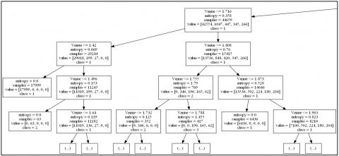
(b). Decision Tree: The decision tree classifier was applied with the “Entropy” criteria with a maximum depth of 25 as the data was large. It scored the highest accuracy for the learning data and predicted class, as shown in Figure 1.
Figure 1. Decision Tree
Table 8. Accuracy of Model for Batting Data
|
Classifier |
Accuracy |
|||
|
60%|40% |
70%|30% |
80%|20% |
90%|10% |
|
|
Naïve Bayes’ |
67.7703 |
67.8193 |
67.5458 |
68.137 |
|
Decision Tree |
97.4492 |
97.4512 |
97.4089 |
97.3407 |
|
Random Forest |
97.071 |
97.139 |
97.182 |
97.248 |
|
SVM |
69.6355 |
69.3076 |
69.6465 |
69.7863 |
Table 9. Accuracy of Model for Batting Data
|
Classifier |
Accuracy |
|||
|
60%|40% |
70%|30% |
80%|20% |
90%|10% |
|
|
Naïve Bayes’ |
91.5327 |
91.4588 |
91.7994 |
91.3459 |
|
Decision Tree |
94.8974 |
94.7866 |
94.9045 |
94.7383 |
|
Random Forest |
94.9078 |
94.7728 |
94.9183 |
94.7314 |
|
SVM |
91.5327 |
91.4588 |
91.7994 |
91.3459 |
(c). Random Forest: Random Forest is the enhanced decision tree with more robust functions. The random forest was modeled with the default number of trees, i.e., 100 estimators. The accuracies were significant as the number of trees was less and increased with higher estimators.
(d). Support Vector Machine: SVM was trained with “rbf” kernel at a random state. It performed lower than expected as the data was huge, but the class labeling did not support the algorithm, and it performed closely to the Naïve Bayes’.
The study produced several significant findings that clarified how well various machine learning algorithms predicted the performance of cricket players. First, the decision tree classifier proved robust and reliable in processing cricket performance data, consistently outperforming competing algorithms across a range of training-test splits. According to this research, decision trees may effectively predict performance outcomes and represent intricate interactions among cricket player traits.
Furthermore, because of the high entropy of the data, the Random Forest classifier was shown to be the best-fit model for the dataset. The Random Forest model's adaptability and effectiveness in capturing complex patterns and variations in player performance across many qualities and settings are highlighted by its capacity to handle high-entropy data. This finding emphasizes how crucial it is to use ensemble learning strategies in sports analytics, such as Random Forest, to improve model performance and forecast accuracy.
Additionally, compared to decision trees and Random Forests, the study found that the Naïve Bayes and SVM classifiers performed comparatively worse. This research implies that decision trees and ensemble approaches may be more successful in forecasting cricket player performance than Naïve Bayes and SVM classifiers, even though they may have certain benefits in particular situations, such as managing smaller datasets or nonlinear connections.
The study's findings highlight how important it is to use ensemble methods and sophisticated machine learning algorithms in sports analytics to enhance player performance prediction and guide managerial and coaching decisions in cricket.
4.1 Implications of the study
This study has implications for sports analytics and cricket management in several areas. First, the suggested framework for evaluating cricket player performance provides an organized methodology that may help managers, coaches, and selectors make well-informed choices about player selection, team composition, and long-term planning. The platform uses machine learning algorithms and sophisticated data preparation techniques to deliver insightful information about player form, consistency, and performance versus certain opponents and settings.
The study's conclusions also benefit the larger area of sports analytics as they show how useful it is to use complex analytical techniques when assessing player performance. An effective framework for deciphering complicated sports data and identifying patterns and trends may be obtained by applying the AHP and ensemble learning algorithms like Random Forest. Consequently, the research emphasizes how crucial it is for sports managers to implement data-driven strategies to improve decision-making and maximize team output.
This research investigated how well different machine learning algorithms could forecast cricket player performance using various characteristics. The results of determining the resilience and reliability of decision tree classifiers in modeling complicated interactions within cricket player data showed that they consistently beat other methods. Furthermore, because of its capacity to handle high-entropy data and recognize complex patterns in player performance, the Random Forest classifier was shown to be the best-fit model for the dataset.
The study did note, however, that the Naïve Bayes and SVM classifiers performed substantially worse than the ensemble techniques and decision trees, indicating that these algorithms may not be as good at predicting the performance of cricket players. The results show the importance of using cutting-edge machine learning methods in sports analytics, including decision trees and Random Forests, to improve forecast accuracy and guide managerial and coaching decisions about cricket.
Future studies may concentrate on enhancing current models and investigating new factors to increase prediction accuracy. Furthermore, exploring deep learning methods and integrating real-time data streams may provide fresh perspectives on the dynamics of player performance and further the development of sports analytics in cricket and other sports.
[1] Ishi, M.S., Patil, J.B. (2020). A study on impact of team composition and optimal parameters required to predict result of cricket match. In Social Networking and Computational Intelligence: Proceedings of SCI-2018. Springer Singapore, pp. 389-399. https://doi.org/10.1007/978-981-15-2071-6_32
[2] Sarangi, S., Singh, R.R. (2023). Winning one-day international cricket matches: A cross-team perspective. Journal of Business Analytics, 6(1): 39-58. https://doi.org/10.1080/2573234X.2022.2041370
[3] Muthuswamy, S., Lam, S.S. (2008). Bowler performance prediction for one-day international cricket using neural networks. In IIE Annual Conference. Proceedings. Institute of Industrial and Systems Engineers (IISE), p. 1391-1395.
[4] Wickramasinghe, I.P. (2014). Predicting the performance of batsmen in test cricket. Journal of Human Sport and Exercise 2014, 9(4): 744-751. https://doi.org/10.14198/jhse.2014.94.01
[5] Barr, G.D.I., Kantor, B.S. (2004). A criterion for comparing and selecting batsmen in limited overs cricket. Journal of the Operational Research Society, 55(12): 1266-1274. https://doi.org/10.1057/palgrave.jors.2601800
[6] Iyer, S.R., Sharda, R. (2009). Prediction of athletes performance using neural networks: An application in cricket team selection. Expert Systems with Applications, 36(3): 5510-5522. https://doi.org/10.1016/j.eswa.2008.06.088
[7] Jhanwar, M.G., Pudi, V. (2016). Predicting the outcome of ODI cricket matches: A team composition based approach. MLSA@ PKDD/ECML, 78.
[8] Lemmer, H.H. (2002). The combined bowling rate as a measure of bowling performance in cricket. South African Journal for Research in Sport, Physical Education and Recreation, 24(2): 37-44. https://hdl.handle.net/10520/EJC108746
[9] Bhattacharjee, D., Pahinkar, D.G. (2012). Analysis of performance of bowlers using combined bowling rate. International Journal of Sports Science and Engineering, 6(3): 184-192.
[10] Mukherjee, S. (2014). Quantifying individual performance in Cricket-A network analysis of Batsmen and Bowlers. Physica A: Statistical Mechanics and its Applications, 393: 624-637. https://doi.org/10.1016/j.physa.2013.09.027
[11] Shah, P. (2017). New performance measure in Cricket. ISOR Journal of Sports and Physical Education, 4(3): 28-30. https://doi.org/10.9790/6737-04032830
[12] Parker, D., Burns, P., Natarajan, H. (2008). Player valuations in the Indian premier league. Frontier Economics, 116: 1-17.
[13] Prakash, C.D., Patvardhan, C., Lakshmi, C.V. (2016). Data analytics based deep mayo predictor for IPL-9. International Journal of Computer Applications, 152(6): 6-10.
[14] Bukiet, B., Ovens, M. (2006). A mathematical modelling approach to one-day cricket batting orders. Journal of Sports Science & Medicine, 5(4): 495-502.
[15] Schumaker, R.P., Solieman, O.K., Chen, H., Schumaker, R.P., Solieman, O.K., Chen, H. (2010). Predictive modeling for sports and gaming. Sports Data Mining, Springer, Boston, MA., 55-63. https://doi.org/10.1007/978-1-4419-6730-5_6
[16] Haghighat, M., Rastegari, H., Nourafza, N., Branch, N., Esfahan, I. (2013). A review of data mining techniques for result prediction in sports. Advances in Computer Science: An International Journal, 2(5): 7-12.
[17] Hucaljuk, J., Rakipović, A. (2011). Predicting football scores using machine learning techniques. In 2011 Proceedings of the 34th International Convention MIPRO, Opatija, Croatia, pp. 1623-1627.
[18] McCullagh, J. (2010). Data mining in sport: A neural network approach. International Journal of Sports Science and Engineering, 4(3): 131-138.
[19] ParseHub. Free web scraping-Download the most powerful web scraper. https://www.parsehub.com/, accessed on Oct. 23, 2023.
[20] Petrović, G., Mihajlović, J., Ćojbašić, Ž., Madić, M., Marinković, D. (2019). Comparison of three fuzzy MCDM methods for solving the supplier selection problem. Facta Universitatis, Series: Mechanical Engineering, 17(3): 455-469. https://doi.org/10.22190/FUME190420039P
[21] Jana, S., Giri, B. C., Sarkar, A., Jana, C., Stević, Ž., & Radovanović, M. (2024). Application of fuzzy AHP in priority based selection of financial indices: A perspective for investors. Economics - Innovative and Economics Research Journal, 12(1): 1-27. https://doi.org/10.2478/eoik-2024-0007
[22] Yousnaidi, R.S., Passarella, R., Kurniati, R., Arsalan, O., Aditya, Afriansyah, I.G., Fathan, M.R., Vindriani, M. (2023). Assessing automatic dependent surveillance-broadcast signal quality for airplane departure using random forest algorithm. Mechatronics and Intelligent Transportation Systems, 2(2): 64-71. https://doi.org/10.56578/mits020202
[23] Kumar, R., Channi, A.S., Kaur, R., Sharma, S., Grewal, J.S., Singh, S., Verma, A., Haber, R. (2023). Exploring the intricacies of machine learning-based optimization of electric discharge machining on squeeze cast TiB2/AA6061 composites: Insights from morphological, and microstructural aspects in the surface structure analysis of recast layer formation and worn-out analysis. Journal of Materials Research and Technology, 26: 8569-8603. https://doi.org/10.1016/j.jmrt.2023.09.127
[24] Quinlan, J.R. (1986). Induction of decision trees. Machine Learning, 1: 81-106. https://doi.org/10.1007/BF00116251
[25] Lou, D., Yang, M., Shi, D., Wang, G., Ullah, W., Chai, Y., Chen, Y. (2021). K-Means and c4. 5 decision tree based prediction of long-term precipitation variability in the Poyang lake basin, China. Atmosphere, 12(7): 834. https://doi.org/10.3390/atmos12070834
[26] Kiran, M.D., BR, L.Y., Babbar, A., Kumar, R., HS, S.C., Shetty, R.P., Sudeepa, K.B., Sampath, K.L., Rupinder, K., Alkahtani, M.Q., Islam, S., Kumar, R. (2024). Tribological properties of CNT-filled epoxy-carbon fabric composites: Optimization and modelling by machine learning. Journal of Materials Research and Technology, 28: 2582-2601. https://doi.org/10.1016/j.jmrt.2023.12.175
[27] Ranjan, N., Kumar, R., Kumar, R., Kaur, R., Singh, S. (2023). Investigation of fused filament fabrication-based manufacturing of ABS-Al composite structures: prediction by machine learning and optimization. Journal of Materials Engineering and Performance, 32(10): 4555-4574. https://doi.org/10.1007/s11665-022-07431-x
[28] Ho, T.K. (1998). The random subspace method for constructing decision forests. IEEE Transactions on Pattern Analysis and Machine Intelligence, 20(8): 832-844. https://doi.org/10.1109/34.709601
[29] Breiman, L. (2001). Random forests. Machine Learning, 45: 5-32. https://doi.org/10.1023/A:1010933404324
[30] Thakur, V., Kumar, R., Kumar, R., Singh, R., Kumar, V. (2024). Hybrid additive manufacturing of highly sustainable Polylactic acid-Carbon Fiber-Polylactic acid sandwiched composite structures: Optimization and machine learning. Journal of Thermoplastic Composite Materials, 37(2): 466-492. https://doi.org/10.1177/08927057231180186
[31] Boser, B.E., Guyon, I.M., Vapnik, V.N. (1992). A training algorithm for optimal margin classifiers. In Proceedings of The Fifth Annual Workshop on Computational Learning Theory, pp. 144-152. https://doi.org/10.1145/130385.130401
[32] Karaoğlu, U., Mbah, O., Zeeshan, Q. (2023). Applications of machine learning in aircraft maintenance. Journal of Engineering Management and Systems Engineering, 2(1): 76-95. https://doi.org/10.56578/jemse020105