Asraa Jalil Saeed*![]() | Ahmed A. Hashim
| Ahmed A. Hashim![]()
© 2024 The authors. This article is published by IIETA and is licensed under the CC BY 4.0 license (http://creativecommons.org/licenses/by/4.0/).
OPEN ACCESS
A Deep Convolutional Generative Adversarial Network (DCGAN) suffers from a vanishing gradient issue in the generator due to the overconfidence of the discriminator. This paper explores the effects of using noise injection and gradually changing label smoothing (CLS) towards hard labels and two-sided label smoothing to enhance the stability of the DCGAN. Different models are trained on CIFAR-10 datasets that contains 60,000 32×32 color images divided into 10 categories and CIFAR-100 datasets that contains 60,000 32×32 color images divided into 100 categories, compared with each other using fréchet inception distance (FID), and Inception Score (IS) evaluation metrics. A noticeable improvement in generalization was found in almost all cases, and the best was when using CLS for both real and fake labels of two-sided smoothing labels. The modified DCGAN performs better than traditional DCGAN, boosting the best fréchet inception distance from 132.31 to 95.52 and the Inception Score (IS) from 25.123 to 64.27 on the CIFAR-10 dataset, the FID from 137.84 to 109.42, and the IS from 19.65 to 61.04 on the challenging CIFAR-100 dataset.
changed smoothing label, DCGAN, noise injection, vanishing gradient issue
Generative Adversarial Networks (GANs) are an important algorithm for generating photorealistic images in computer vision. GAN has gained wide popularity and attention since its invention in 2014 [1]. Its general architecture consists of two competing networks, one of which is the generator and the other is the discriminator [2]. The DCGAN is a type of GAN used in several areas, such as generating images, text-to-image translation, and image-to-image translation [3, 4].
In 2015, DCGAN was introduced by Alec Radford as an innovation in GANs using convolutional neural networks (CNNs) in order to contain convolutional layers similar to CNN layers [5]. CNNs, known for using convolutional layers, are state-of-the-art in most computer vision applications [6].
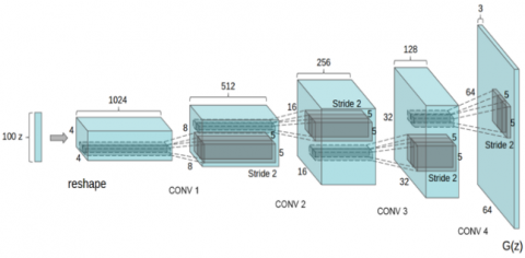
Figure 1. The generator’s architecture of DCGAN [5]
The architecture of the generator is shown in Figure 1, there are four deconvolution layers, the kernel size is 5×5 and the stride is 2 for each layer [5].
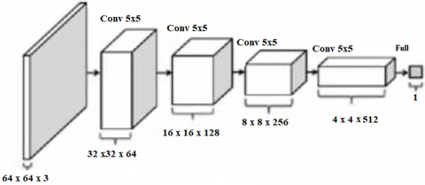
While the discriminator has four convolution layers with last layer is fully connected as shown in Figure 2, the kernel is also 5×5 and stride is 2. This model of DCGAN is applied on the LSUN bedrooms, and FACES dataset [5].
Figure 2. Discriminator’s architecture of DCGAN [7]
Radford added batch normalization at each layer, which stabilizes the training process [8]. The ReLU activation function was used for hidden layers, Tanh for the final layer in the generator, and Leaky ReLU (0.2) for the discriminator [9]. Due to the DCGAN architecture, built on CNNs, leaky ReLU activation, batch normalization, and other key design choices, offers significant advantages over traditional GANs. It’s stability, high-quality image generation, scalability, and wide applicability make it a powerful tool for various tasks in generative modeling, as it allows the model to learn hierarchical features from the data [10]. However because the sub-networks (generator and discriminator) are competitive and they both try to reduce their own loss functions as much as possible, DCGAN still suffers from instability [11]. There are three main causes of instability: non-convergence, vanishing gradients, or mode collapse, viewed as a problem [12]. The vanishing gradients problem may happen when the discriminator is overconfident, especially at the beginning of training, which leads to squashing the gradients of the generator [13]. Table 1 illustrates the explanation of each cause and how they relate to the stability issue in DCGANs.
Table 1. The instability issue in DCGANs
|
Cause of Instability |
Explanation |
Relation to Stability in DCGANs |
|
Vanishing or Exploding Gradient Problem |
The vanishing means that the gradients get smaller, and the weight updates generated by the optimization process may likewise become very small. This results in minimum weight modifications throughout training. |
The issue occurs during backpropagation, it is difficult to update the weights efficiently, which might significantly slow down or hinder the training process. So Ineffective weight updates cause slow or unstable training. |
|
Mode Collapse Problem |
Generators create a limited number of samples, which results in a lack of variety. |
The limited diversity of generated samples influences stability. |
|
Non-Convergence Problem |
This problem occurs due to the min-max game that is used as a loss function; it is neither convex nor concave, which leads to oscillation and divergence of the generator and discriminator during training. |
Batch normalization is critical for maintaining stability and improving convergence. |
|
Overconfidence of the Discriminator |
An overconfident discriminator tends to provide gradients close to zero to the generator, which might result in vanishing gradients and restrict the generator's learning. The generator might be unable to enhance its ability to provide realistic samples. |
The discriminator in DCGANs can become overconfident, especially in the early stages of training when it hasn't yet seen a diverse set of real and generated samples. |
DCGAN faces challenges such as the vanishing gradient problem, which impedes effective training by causing slow convergence or stagnation. This issue is particularly relevant for both the generator and discriminator networks.
The other challenge for the DCGAN is overconfident discriminator, consider the generator as an artist working under the discriminator's criticism to create a work of art. The discriminator's feedback must pass across network layers and return to the generator during training. However, these gradients tend to vanish, leaving the generator with warped and feeble instructions, like whispers in a long corridor.
Several techniques, like label smoothing, dropout in the discriminator, noise injection to the discriminator, or adjusting the loss functions, which help keep consistency during training [14, 15], are effective at alleviating overconfidence in the GAN's discriminator and instability.
The objectives of this paper are to make DCGAN more stable by adding two techniques together with DCGAN to address the overconfidence of the discriminator: using noise injection, and gradually changing label smoothing (CLS).
There are two types of smoothing labels that alleviate the over-confidence of the discriminator: one-sided and two-sided label smoothing. The term "one-sided label smoothing" refers to the method used by Ian in his 2016 article [16], which included substituting the real target values with a fraction of a true one, say, 0.9. While Salman used this technique in the same year but with positive and negative smoothing values [17], by using $\propto, \beta$ in Eq. (1):
$D(x)=\left(\propto p_{\text {data }}(x)+\beta p_{\text {model }}(x)\right) /\left(p_{\text {data }}(x)+p_{\text {model }}(x)\right)$ (1)
where, pdata represents the probability of the real distribution that is close to 0 and pmodel represents the probability of the generated distribution that is large and therefore causing the problem, therefore smoothing only the positive labels $\propto$, having zeros for negative labels.
One potential weakness of one-sided label smoothing is the potential loss of discriminative power in the discriminator. In GANs, the discriminator's role is crucial in distinguishing between real and generated samples. Label smoothing involves assigning less extreme labels to real samples, essentially introducing some level of uncertainty or ambiguity [18].
While this can prevent the generator from becoming overly confident, it might also make the discriminator less effective at accurately discerning real data from generated data [19].
In 2021, the effect of noise and stochastic two-sided label smoothing on model convergence is investigated in Zhang [20]'s article. This may provide improved solutions to the vanishing gradient problem and more regularizing effects than the one-sided approach.
In general, label smoothing is a simple, effective regularization approach to overcome the overfitting issue with the training set distribution in any deep neural network.
Although such label smoothing can provide excellent regularization and keep trained models from becoming overconfident, it is treated by assigning them the same fixed probability. As a result, the probability assigned to the generated samples should take into account their similarities to the real sample; treating may limit the diversity of the generated samples, influence stability, and restrict the model's effectiveness [20].
In the early stages of GAN training, the discriminator is typically overconfident due to the limited data available. This can prevent the generator from learning effectively. Smoothing labels, which assign real and fake labels with probabilities (0.9, 0.1) instead of binary values, can help address this problem by providing the generator with more nuanced feedback.
So we propose a novel approach, starting with a smoothing label of 0.9 for real samples and 0.1 for fake samples. As training progresses, we gradually reduce the smoothing factor by a small value (0.001) at each iteration.
Noise injection was first utilized to address overfitting in deep learning networks [15]; more recently, it has been connected with GAN to address instability [21-23]. Noise injection is also utilized to create high-resolution images especially if injected into the generator at each layer [24]. In this paper, a proposed noise injection to the discriminator of the DCGAN was used to enhance stability with all scenarios.
Injecting noise into the discriminator's input to penalize the gradients of the discriminator and makes it more resilient to variations in the input data.
Table 2. Summary of noise injection with pros and cons
|
Noise injection with |
Network Type |
Reference |
Pros |
Cons |
|
Deep learning |
[15] |
Address overfitting |
Slow down the convergence. |
|
|
The generator |
[23, 24] |
High-resolution images + Reduces GAN vulnerability |
Better for modest-size training sets + it still faces a trade-off between stability and generation quality. |
|
|
Adaptive, and tune the noise with the discriminator (modulation of features via multiplicative noise) |
[22] |
Improves stability |
Doesn't elaborate on how to optimally tune the noise attributes (distribution, variance). Finding the right settings might require experimentation and potentially be data-dependent. |
|
|
The discriminator |
[21] |
Improves stability and convergence during GAN training |
Diffusion-GAN computationally expensive, particularly during the training phase +sensitive to the choice of hyperparameters, such as the number of diffusion steps, noise schedule, and generator architecture. |
|
|
The discriminator's input |
Our work |
Increase diversity, Stability, mitigate mode collapse, overconfident discriminator |
Complement with smoothing labels together to give a better results. |
The main reasons why injecting noise technique is used in the discriminator not in the generator is due to the regularization, stability during training, increasing diversity, and mitigating mode collapse, which could be seen in Table 2.
To inhibit the discriminator, a novel smoothing technique (CSL) was used as follows:
(1) The real label was changed gradually, starting at 0.9 instead of 1 and increasing gradually by 0.001 until reaching 1. (0.9, 0.901, 0.902, …, 1).
(2) Changed gradually smooth labels with both real and fake labels, starting from 0.9 for the real label and increasing gradually by 0.001, and 0.1 for the fake label and decreasing gradually by 0.001 until it reached 0. (0.1, 0.099, 0.098, ..., 0).
(3) This technique was used on the CIFAR-10 and CIFAR-100 datasets for 200 iterations. When reaching 100 iterations, the real and fake labels became 1 and 0, respectively.
Now that we have passed the beginning of training and the discriminator has become more accurate, we will try to utilize the hard label (0 and 1) or soft label (0.1 and 0.9) values to collect and evaluate several answers objectively. All methods above use noise injection simultaneously to the discriminator that reduces the euclidean case of the distribution.
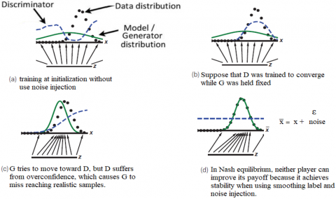
Figure 3. (a) The discriminator at initial training, (b) The generator is unable to enhance its ability to provide realistic samples, (c) Overconfidence of the discriminator, (d) When use noise injection with input the discriminator. x is real data, z is noise vector, $\bar{x}$ is input real with some epsilon noise, (ε) The discriminator function (D blue line), dot black curve is real data distribution, green line is fake data distribution
Five layers of transpose convolution for the generator were built and then ReLU was utilized as an activation function in the four layers and Tanh in the final layer. The kernel size that is used in each layer is [4×4], while the discriminator is built with five layers of convolution. After each layer, there is LeakyReLU with slop (0.2), except the final layer has sigmoid to attain classification (0 or 1), 0 for fake, and 1 for the real image. Batch normalization (BN) was added before activation functions ReLU and LeakyReLU to maintain stability. Table 3 illustrates the architecture of DCGAN.
A deep examination of the impact of the gradually changed label smoothing (CLS) application in multiple scenarios and considering DCGAN without smoothing labels as a benchmark to compare all scenarios and know the best approach with the CIFAR-10 and CIFAR-100 datasets. The noise was injected into the discriminator to increase stability.
Table 3. The architecture of modified DCGAN for generating 64×64 images
|
Generator |
Stride |
Padding |
Output Shape |
|
Input |
— |
— |
100×1×1 |
|
ConvTranspose + ReLU |
1 |
0 |
512×4×4 |
|
ConvTranspose + BN + ReLU |
2 |
1 |
256×8×8 |
|
ConvTranspose + BN + ReLU |
2 |
1 |
128×16×16 |
|
ConvTranspose + BN + ReLU |
2 |
1 |
64×32×32 |
|
ConvTranspose + Tanh |
2 |
1 |
3×64×64 |
|
Discriminator |
|
|
|
|
Input |
— |
— |
3×64×64 |
|
Convolution + LeakyReLU |
2 |
1 |
64×32×32 |
|
Convolution +BN + LeakyReLU |
2 |
1 |
128×16×16 |
|
Convolution +BN + LeakyReLU |
2 |
1 |
256×8×8 |
|
Convolution +BN + LeakyReLU |
2 |
1 |
512×4×4 |
|
Convolution + Sigmoid |
1 |
0 |
1 |
Injecting noise prevents the discriminator from overfitting to specific data patterns; this helps it generalize better, enhances its ability to handle variations in the generated samples, and prevents it from becoming too confident in its predictions and potentially diverging during the adversarial training process. Injecting noise with the discriminator makes it harder for the discriminator to exploit specific patterns consistently. Figure 3 shows how training is more stable when using noise in the input of the discriminator.
Fréchet inception distance (FID) [25] and Inception Score (IS) [17] are commonly metrics that evaluate generative algorithms. In 2016, Salimans and his colleagues created the inception score (IS). Before creating the IS metric, humans are left to see a generative image and provide a visual assessment of it. Still, these assessments are subjective and prone to significant variation depending on the viewer's tastes and prejudices. The IS metric's score can be anywhere from worst (0) to best (∞) [17]. Eq. (2) describes how the IS score is calculated:
$\mathrm{IS}(\mathrm{G})=\exp (E x \sim p g D K L(p(y \mid x) \| \mathrm{p}(\mathrm{y})))$ (2)
where, DKL is Kullback-Leibler divergence, the conditional probability distribution is p(y|x), the marginal probability distribution is p(y), Ex~pg is the sum and average of all results.
In 2017, fréchet inception distance (FID) is used as a measure of the similarity of synthetic images to real ones better than the Inception Score (IS) [25]. The FID is a similarity metric between curves that accounts for the position and sequence of points on the curves. Additionally, it may be used to determine the distance between two distributions [26], and it is more consistent with evaluating human vision, so it was used in this article to find out how much image quality improves when stability is improved [27]. When the FID value is low, the distance between the generated and actual data distributions is small, indicating high-quality and diverse images [28]. Eq. (3) describes how the FID is calculated [29]:
$F I D(r, g)=\|\mu r-\mu g\|^2-\operatorname{Tr}\left(\sum r+\sum g-2 * \sqrt{\sum r+\sum g}\right)$ (3)
where, μr and μg are the means array, Tr is the trace of the matrix, and $\sum \mathrm{r}$ and $\sum \mathrm{g}$ is the covariance array of the vectors. In this paper, FID was used to test quality-generated images using improved DCGAN, which means more quality images have stability training. The loss function curve for both the network generator and discriminator was also drawn in this work to see the convergence and oscillation of training.
The trained approach produces 64×64-pixel images. Both the discriminator and the generator have their learning rates set to the default values of 0.0003 and 0.0001, respectively. 200 training epochs are used for the CIFAR-10 and CIFAR-100 datasets. For all models, the Adam optimizer with β1=0.5 and β2=0.999 was used for training.
The first case is a benchmark for constructing DCGAN without the use of a smoothing label and noise injection. The second scenario is when using 0.9 for the real label and 0.1 for the fake label due to the overconfidence of the discriminator at the beginning of the training, and then increasing and decreasing the real and fake labels at the same time by 0.001. That’s to say, after 100 iterations the real and fake labels will become hard labels (0, 1). In this situation, there are two scenarios for testing, the first approach stays on the hard label until we finish the training, and the second approach converts to a two-sided smoothing label with 0.9 for real and 0.1 for fake.
The third trained the same way as the second approach, but with a real label only at 0.9 and increasing gradually until access to the 100 epoch, and here there are two ways, one towards the hard label and the other towards the one-sided smoothing label. The same scenarios were applied to the second dataset, as shown in Table 4, which shows that the FID, and IS metrics of modified DCGAN perform better with CSL and noise injection.
Table 4. FID score comparison with a changed smoothing
|
Scenario |
Method |
CIFAR-10 |
CIFAR-100 |
||
|
FID |
IS |
FID |
IS |
||
|
1 |
DCGAN without a smoothing label and no noise injection (NI) (traditional DCGAN) |
132.31 |
25.123 |
137.84 |
19.65 |
|
2 |
DCGAN + NI+ CSL (real and fake labels) + hard label (1, 0) |
111.43 |
46.89 |
113.20 |
42.62 |
|
3 |
DCGAN + NI + CSL (real and fake labels) + two-sided smoothing label (0.9, 0.1) (Best CLS) |
95.52 |
64.27 |
109.42 |
61.04 |
|
4 |
DCGAN + NI+ CSL (real only) + hard label (1) |
104.03 |
52.11 |
114.26 |
48.21 |
|
5 |
DCGAN + NI+ CSL (real only) + one-sided smoothing label (0.9) |
104.87 |
58.29 |
112.54 |
54.29 |
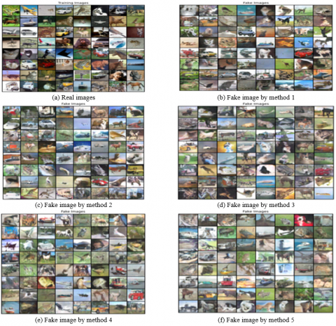
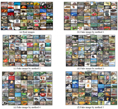
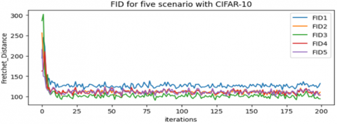
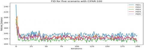
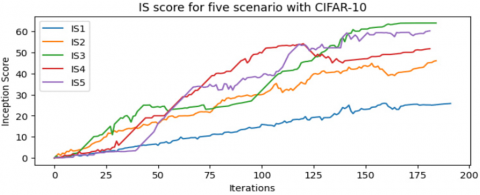
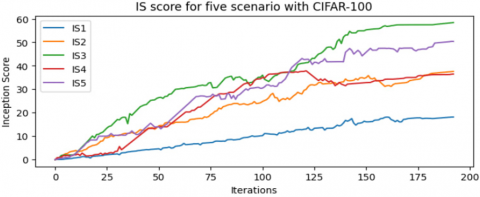
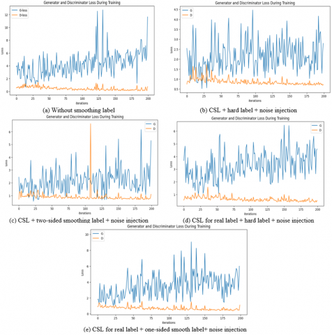
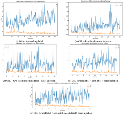
A modified DCGAN shows better performance than traditional DCGAN in all scenarios, significantly in the Best CLS scenario as illustrated in Table 4, with a lower FID (95.52) on the CIFAR-10 dataset and a lower FID (109.42) on the CIFAR-100 dataset, and with best IS (64.27) on the CIFAR-10 dataset and a best IS (61.04) on the CIFAR-100 dataset. Figure 4 and Figure 5 illustrate that the modified DCGAN can better generate samples that approximate the original image. Figures 6 and 7 show how the FID curves decrease, and Figures 8 and 9 show how the IS curves increase with a modified DCGAN for all scenarios throughout the training. In Figures 10 and 11, you can see that convergence got better by looking at the loss functions for both the network generator and the discriminator. These loss functions show convergence and oscillation of training.
Figure 4. Comparisons of images generated with real images by different methods using CIFAR-10
Figure 6. FID curves for the five methods in Table 4 use CIFAR-10
Figure 7. FID curves for the five methods in Table 4 use CIFAR-100
Figure 8. IS curves for the five methods in Table 4 use CIFAR-10
Figure 9. IS curves for the five methods in Table 4 use CIFAR-100
Figure 10. Loss function curves for discriminator and generator, use the CIFAR-10 dataset
Figure 11. Loss function curves for discriminator and generator, use the CIFAR-100 dataset
In this paper, a modified DCGAN incorporates a novel technique called Changed Label Smoothing and also uses noise injection in the discriminator. These techniques, when combined, will alleviate the overconfidence of the discriminator that affects the training of the generator, so they will address the vanishing gradient problem.
The modified DCGAN achieves this performance on the CIFAR-10 and CIFAR-100 datasets. Although both the CIFAR-10 and CIFAR-100 datasets include the same features, such as 60,000 32×32 color images, the best results were achieved using CIFAR-10. The reason for that is because they differ in number and kinds of classes. The proposed approach (Changed Label Smoothing) may be applied in other GAN architectures or may be combined with other techniques.
[1] Arora, J., Tushir, M., Kherwa, P., Rathee, S. (2023). Generative adversarial networks: A comprehensive review. Data Wrangling: Concepts, Applications and Tools, 213-234. https://doi.org/10.1002/9781119879862.ch10
[2] Liu, G., Liu, Y., Tang, L., Bavirisetti, D.P., Wang, X. (2023). A Generative Adversarial Network for infrared and visible image fusion using adaptive dense generator and Markovian discriminator. Optik, 288: 171139. https://doi.org/10.1016/j.ijleo.2023.171139
[3] Kaddoura, S. (2023). Real-world applications. In A Primer on Generative Adversarial Networks, pp. 27-81. https://doi.org/10.1007/978-3-031-32661-5_3
[4] Rasheed, A.S., Finjan, R.H., Hashim, A.A., Al-Saeedi, M.M. (2021). 3D face creation via 2D images within blender virtual environment. Indonesian Journal of Electrical Engineering and Computer Science, 21(1): 457-464. https://doi.org/10.11591/ijeecs.v21.i1.pp457-464
[5] Radford, A., Metz, L., Chintala, S. (2015). Unsupervised representation learning with deep convolutional generative adversarial networks. arXiv preprint arXiv:1511.06434. https://arxiv.org/abs/1511.06434
[6] Quiroga, F.M. (2021). Invariance and same-equivariance measures for convolutional neural networks. CLEI Electronic Journal, 24(1): 8. https://doi.org/10.19153/cleiej.24.1.8
[7] Bushra, S.N., Maheswari, K.U. (2021). Crime investigation using DCGAN by Forensic Sketch-to-Face Transformation (STF)-A review. In 2021 5th International Conference on Computing Methodologies and Communication (ICCMC), pp. 1343-1348. https://doi.org/10.1109/ICCMC51019.2021.9418417.
[8] Finjan, R.H., Rasheed, A.S., Hashim, A.A., Murtdha, M. (2021). Arabic handwritten digits recognition based on convolutional neural networks with resnet-34 model. Indonesian Journal of Electrical Engineering and Computer Science, 21(1): 174-178. https://doi.org/10.11591/ijeecs.v21.i1.pp174-178
[9] Liu, B.Q., Lv, J.W., Fan, X.Y., Luo, J., Zou, T.Y. (2022). Application of an improved DCGAN for image generation. Mobile Information Systems, 2022: 9005552. https://doi.org/10.1155/2022/9005552
[10] Wu, A.N., Stouffs, R., Biljecki, F. (2022). Generative adversarial networks in the built environment: A comprehensive review of the application of GANs across data types and scales. Building and Environment, 223, 109477. https://doi.org/10.1016/j.buildenv.2022.109477
[11] Kumar, J.K. (2022). Alma mater studiorum-università di bologna. School of engineering and architecture.
[12] Wiatrak, M., Albrecht, S.V., Nystrom, A. (2019). Stabilizing generative adversarial networks: A survey. arXiv preprint arXiv:1910.00927. https://doi.org/10.48550/arXiv.1910.00927
[13] Saeed, A.J., Hashim, A.A. (2023). Precise GANs classification based on multi-scale comprehensive performance analysis. Journal of Engineering Science & Technology Review, 16(3): 18. https://doi.org/10.25103/jestr.163.18
[14] Zhong, H., Yu, S., Trinh, H., Lv, Y., Yuan, R., Wang, Y. (2023). Fine-tuning transfer learning based on DCGAN integrated with self-attention and spectral normalization for bearing fault diagnosis. Measurement, 210: 112421. https://doi.org/10.1016/j.measurement.2022.112421
[15] Chu, X., Zhang, B. (2020). Noisy differentiable architecture search. arXiv preprint arXiv:2005.03566. https://arxiv.org/abs/2005.03566
[16] Goodfellow, I. (2016). Nips 2016 tutorial: Generative adversarial networks. arXiv preprint arXiv:1701.00160. https://doi.org/10.48550/arXiv.1701.00160
[17] Salimans, T., Goodfellow, I., Zaremba, W., Cheung, V., Radford, A., Chen, X. (2016). Improved techniques for training GANS. Advances in neural information processing systems, 29. https://proceedings.neurips.cc/paper_files/paper/2016/file/8a3363abe792db2d8761d6403605aeb7-Paper.pdf.
[18] Chandrasegaran, K., Tran, N.T., Zhao, Y., Cheung, N.M. (2022). Revisiting label smoothing and knowledge distillation compatibility: What was missing?. In International Conference on Machine Learning, pp. 2890-2916. https://doi.org/10.3390/app11104699
[19] Szegedy, C., Vanhoucke, V., Ioffe, S., Shlens, J., Wojna, Z. (2016). Rethinking the inception architecture for computer vision. In Proceedings of the IEEE conference on computer vision and pattern recognition, pp. 2818-2826. https://doi.org/10.1109/cvpr.2016.308
[20] Zhang, C.B., Jiang, P.T., Hou, Q., Wei, Y., Han, Q., Li, Z., Cheng, M.M. (2021). Delving deep into label smoothing. IEEE Transactions on Image Processing, 30: 5984-5996. https://doi.org/10.36227/techrxiv.22714999
[21] Wang, Z., Zheng, H., He, P., Chen, W., Zhou, M. (2022). Diffusion-GAN: Training GANs with diffusion. arXiv preprint arXiv:2206.02262. https://doi.org/10.48550/arXiv.2206.02262
[22] Ni, Y., Koniusz, P. (2024). NICE: NoIse-modulated consistency regularization for data-efficient GANs. Advances in Neural Information Processing Systems, 36.
[23] Arjovsky, M., Bottou, L. (2017). Towards principled methods for training generative adversarial networks. arXiv preprint arXiv:1701.04862. https://arxiv.org/pdf/1701.04862.pdf
[24] Feng, R., Zhao, D., Zha, Z.J. (2021). Understanding noise injection in GANs. In international conference on machine learning, pp. 3284-3293. https://ar5iv.labs.arxiv.org/html/2006.05891
[25] Heusel, M., Ramsauer, H., Unterthiner, T., Nessler, B., Hochreiter, S. (2017). Gans trained by a two time-scale update rule converge to a local nash equilibrium. Advances in neural information processing systems, 30. https://doi.org/10.18034/ajase.v8i1.9
[26] Lee, J., Lee, M. (2023). FIDGAN: A generative adversarial network with an inception distance. In 2023 International Conference on Artificial Intelligence in Information and Communication (ICAIIC). https://doi.org/10.1109/icaiic57133.2023.10066964
[27] Andreou, I., Mouelle, N. (2023). Evaluating generative adversarial networks for particle hit generation in a cylindrical drift chamber using fréchet inception distance. Journal of Instrumentation, 18(06): P06007. https://doi.org/10.1088/1748-0221/18/06/p06007
[28] Zhang, H., Xu, T., Li, H., Zhang, S., Wang, X., Huang, X., Metaxas, D.N. (2018). Stackgan++: Realistic image synthesis with stacked generative adversarial networks. IEEE Transactions on Pattern Analysis and Machine Intelligence, 41(8): 1947-1962. https://doi.org/10.1109/tpami.2018.2856256
[29] Nunn, E.J., Khadivi, P., Samavi, S. (2021). Compound frechet inception distance for quality assessment of gan created images. arXiv preprint arXiv:2106.08575. https://arxiv.org/abs/2106.08575