Punitha Aneetchan*![]() | Geetha Vaithianathan
| Geetha Vaithianathan![]()
© 2024 The authors. This article is published by IIETA and is licensed under the CC BY 4.0 license (http://creativecommons.org/licenses/by/4.0/).
OPEN ACCESS
In the agricultural sector, soil quality plays a pivotal role in determining crop types. Traditional manual soil analysis can be time-consuming and reliant on a limited number of experts, often resulting in insufficient knowledge about local soil conditions. For accurate soil classification process, this study develops a Dwarf Mongoose Optimization with DL Based Soil Classification (DMODL-SC) model. The presented DMODL-SC technique majorly recognizes different kinds of soil using CV and DL models. In the presented DMODL-SC technique, bilateral filtering (BF) technique is used for noise removal process which eradicate the presence of noise exist in the soil images and enhances its quality. In addition, the presented DMODL-SC technique employs capsule network (CapsNet) model for feature extraction process. Moreover, Denoising Auto Encoder (DAE) is exploited for the identification and classification of soil. Since the manual hyperparameter tuning is a tedious process, the DMO algorithm is applied to tune the hyperparameters related to the DAE model. To demonstrate the enhanced performance of the projected DMODL-SC system, an extensive range of experiments were performed. The comparison study reported the improvised soil classification performance of the DMODL-SC technique over other approaches with maximum accuracy of 95.92%.
soil classification, computer vision, artificial intelligence, precision agriculture, DL
Precision agriculture allows precise consumption of inputs like fertilizers, seed, water, and pesticides timely for the crop to maximize quality, yields, and productivity [1, 2]. By deploying sensors for mapping fields and data collection, farmers could understand the field in a better way conserve the resource being used, and decrease adversarial effects on the environment. Mostly, the farmers practice outdated farming patterns for deciding on crops to be cultivated in the field [3]. But the farmer doesn’t perceive crop yields as interdependent on climatic conditions and soil characteristics. Forecasting the variety of crops in specific regions is a challenging and very difficult task since it is influenced by the climatic parameters and type of soil [4]. Moreover, the crop is based on the type of technique utilized by farmers in field-to-field, thus forecasting the performance of Crop types in the parametric perspective is challenging. With the growing population, it exists a substantial demand for crops worldwide [5]; therefore, farmer needs that aware of crop variety which is fixable to the soil type and geographical location [6]. Thus, there is a need for providing timely-based, accurate data according to the soil type to the farmers and climatic parameters, helping them make better decisions for their soil, resulting in great productivity and profitability [7].
Climatic parameters like, precipitation, sunlight, temperature and humidity employ a reflective effect on crop yields. Their complex interaction directly influences crop progress, improvement as well as complete productivity. Temperature affects amount of plant development and flowering while precipitation ranks are serious for sufficient soil moisture. Sunlight and humidity are vital for photosynthesis as well as creation of plant structures [7]. But, huge challenge in predicting crop yields lies in complex nature of weather parameters, their temporal and spatial variations, nonlinear relations among these aspects and crop results. Furthermore, weather change presents extra irregularity that makes complex to accurately expect how shifts in climatic situations will influence prospect crop yields that highlighting requirement for advanced modeling as well as data-driven techniques in agricultural estimating. The superior of accurate crop variety is dominant in enhancing agricultural harvest. Dissimilar crop variations varying acceptance levels for exact environmental circumstances, types of soil and geographical areas.
Soil plays a vital part in hydrologic sequence by performing as a reservoir for water and simplifying its effort via landscape. The soil's capability is to grip and relief water effects availability for crops, surface runoff and groundwater recharge. Soil assets and their relations with vegetation and precipitation command its part in changeable water quality and flow. Modeling surface excess is vital to water and soil conservation efforts as it aids to forecast water movement across scenery. Surface runoff techniques consider causes like vegetation cover, type of soil, topography, and precipitation to pretend water movement paths and recognize prospective sedimentation and erosion threats. By evaluating and modifying surface runoff, land managers and conservationists can able to decrease soil erosion, guard water excellence, and improve complete sustainability in environmental and agricultural situations. Flooding and Erosion caused by uncontrollable runoff, mostly down-stream, cause damage to agricultural land and manmade structure [8]. Consequently, modelling surface runoff is a critical part of soil and water conservation effort including but has not been constrained to, predictive floods, and monitoring soil, soil erosion, and water quality [9]. Soil could be classified into silty sand, clayey sand, sandy clay, humus clay, clay, clayey peat, and peat. Numerous soil classifier techniques are presented in this work. The boundary and signal energy model for feature extraction [10].
This study develops a Dwarf Mongoose Optimization with DL Based Soil Classification (DMODL-SC) model. The presented DMODL-SC technique majorly recognizes different kinds of soil using CV and DL models. In the presented DMODL-SC technique, bilateral filtering (BF) technique is used for noise removal process. In addition, the presented DMODL-SC technique employs capsule network (CapsNet) model for feature extraction process. Moreover, DMO with denoising auto encoder (DAE) is exploited for the identification and classification of soil. To demonstrate the enhanced performance of the projected DMODL-SC system, an extensive range of experiments were performed.
Xiao et al. [11] devise an ML technique for integrating the CPTU data and borehole in a rigorous Bayesian structure and identifying and separating noisy CPTU data without subjective judgments that give to add reliable property evaluation and soil classifier. The CPTU data and borehole-reported soil types will be treated as 2 kinds of evidence of authentic soil types. Shivhare and Cecil [12] formulated a mechanism for classifying the soil at their optimum attempt through extraction of its nature and features. The mechanism will use Gabor Wavelet and SVM to recognize soil variety and categorize for superior recommendation.
In the study [13], the authors sightsee a liquid crystal tunable filter (LCTF)-related mechanism and devise a 3D-CNN for soil classifications. The research scholars initially gain a group of soil compressing measurements through lower spatial resolution detectors, and soil hyperspectral imageries were rebuilt with enhanced resolution from the spatial along with the spectral domains through compressive sensing (CS) technique. In the study [14], the authors have created cloud-related agricultural structure that empowers Indian agriculturalists, agro industries, and agricultural departments for extracting valuable agricultural data. The modelled agricultural cloud structure offers 2 services they are crop yield prediction as a service and soil classification as service. In order to classifier of soil, hybrid SVM (M-SVM) and for wheat yield forecast, modified ANN (M-ANN) has been formulated.
Bouayad et al. [15] modelled enforcement of the Gaussian mixture (GM) technique for classifier of the soil utilizing several cone penetration tests (CPT). The GM method will categorize the CPT data through indication of probability density function. A GM method related expectation maximization (EM) technique includes Bayesian information criterion (BIC) to select optimum count of clusters was formulated through 6 real CPT data. Radhika and Madhavi Latha [16] introduce a complete classifier technique for classifying soil textures by utilizing Linear Discriminant Analysis (LDA). The authors would take the Physico-chemical property of soils including potassium, soil moisture, power conductivity, temperature, available nitrogen, pH, accessible phosphorus, and organic carbon, as independent variables, whereas type of soil will be considered as the dependent variable.
An important study of DL-Based Soil Classification techniques is vital essential for complete hyperparameter tuning. DL models shown extraordinary potential in soil detection, optimum structure of hyperparameters remains a serious but frequently ignored feature of model improvement. The excellent of hyperparameters contains batch sizes, learning rates, regularization methods, network designs which considerably effects a model's performance. A detailed fine-tuning and exploration of these hyperparameters leads to enhanced model accurateness, simplification, and sturdiness that finally improves practical applicability of these techniques in everyday farming and environmental situations. This study gap is vital for connecting complete potential of DL in soil classification as well as addressing most difficult challenges in exactness farming and land organization.
3.1 Image pre-processing
In the presented DMODL-SC technique in Figure 1, the BF technique is used for noise removal process. The BF approach offers the advantage of automated censoring, less noise, rotation symmetric, and ease to design [17]. The input image may have noises, involving salt pepper noise, Gaussian, etc. Noise removal application preserves the information on the input data similarly. The BF method is employed for denoising the input images. This is accomplished by integrating two Gaussian filters, viz., the spatial domain, another one that operates the intensity domain, and the one that is functioning. The resultant at $p$ pixel place was determined as:
$\bar{F}\left( p \right)=\frac{1}{N}\mathop{\sum }_{z\epsilon S\left( p \right)}e\frac{-\|q-p{{\|}^{2}}}{2\varepsilon _{e}^{2}}\frac{-|F\left( q \right)-F\left( p \right){{|}^{2}}}{2\mathcal{E}_{S}^{2}}F\left( q \right)$ (1)
Now, the normalization constant is denoted by $N$, $S\left( p \right)$ characterize a pixel spatial neighborhood $F\left( p \right)$, and variable ${{\varepsilon }_{e}}{{\varepsilon }_{r}}$ are governing weightedin the domain of spatial and intensity begin with fall off.
${{e}^{\frac{-\|q-p{{\|}^{2}}}{2\varepsilon _{e}^{2}}}}{{e}^{\frac{-|F\left( q \right)-F\left( p \right){{|}^{2}}}{2\varepsilon _{e}^{2}}}}$ (2)
The BF was employed in texture removal, tone mapping, volumetric de‐noising, and another application like de‐noising the image is utilized. They could produce simpler conditions for downsampling the procedure and accomplish acceleration by demonstrating in the augmented space; with 2 nonlinearities, the BF has been implemented as linear convolutional.
Figure 1. Block diagram of DMODL-SC system
3.2 Feature extraction using CapsNet
At this stage, the presented DMODL-SC technique employed the CapsNet model for feature extraction process. A primary advantage of CapsNet is that holds the features of further concrete characteristics that aretakenfor understanding how and what is the network learning. The CapsNet can able to encode spatial information and distinguish amongst different orientations, poses, and textures [18]. The capsule is a collection of neurons, thereby each capsule has an activity vector interconnected with it that captures many instant parameters to recognize specific type of object or its part. The orientation and length of vector presented the possibility or probability of existence of that object and the generalization pose. This vector was passed onto the upper level capsule in lower layer capsule. The coupling coefficient occurs amongst the capsule layers. Once the prediction by the lower level capsule equals the result of existing capsule, the values of coupling coefficient amongst them increase, computed by using softmax function. Particularly, once the existing capsule recognizes a tight cluster of previous prediction, and intensely represent the existence of that object, its results in a high probability are also identified as routing by agreement. Figure 2 illustrates the architecture of CapsNet module:
${{\hat{u}}_{{{j}_{|i}}}}\wedge ={{W}_{ij}}{{u}_{i}}$ (3)
In Eq. (3), ${{\hat{u}}_{{{j}_{|i}}}}$ represent the results of prediction vector of upper‐level ${{j}^{th}}$ capsules, ${{W}_{ij}}$ and ${{u}_{i}}$ indicates the weight matrixes and prediction vector of $i$-$th$ capsules in lower layer. It captures spatial connection and interaction amongst objects and sub‐objects. In Eq. (4), based on degree of agreement among nearby layer capsules, the coupling coefficient was evaluated by means of softmax function:
${{c}_{ij}}=\frac{exp\left( {{b}_{ij}} \right)}{\sum exp\left( {{b}_{ik}} \right)}$ (4)
where,${{b}_{ij}}$ indicates the$~log$ probability among 2 capsules, initialization to 0, and $k$ denotes the capsule count. The input vector ${{s}_{j}}$ to ${{j}^{th}}$ layer capsules that a weight sum of ${{\hat{u}}_{{{j}_{|i}}}}\wedge $ vector learned by routing method is calculated by the following equation:
${{s}_{j}}=\underset{i}{\mathop \sum }\,{{c}_{ij}}{{\hat{u}}_{{{j}_{|i}}}}$ (5)
Finally, a squashing purpose which incorporates squashing and unit scaling (Eq. (6)) was implemented for restraining the value of outcomes in the range among [0, 1], thus evaluating the probability as:
$\|{{s}_{j}}{{\|}^{2}}{{v}_{j}}=\underline{1+\|{{s}_{j}}{{\|}^{2}}}\frac{{{s}_{j}}}{{{s}_{j}}}$ (6)
The loss function (interconnected to capsule from the concluding layer, while $m+ar\iota d$ m‐ are set as 0.9 and 0.1 resp.
${{l}_{k}}={{T}_{k}}\text{max}{{(0,~{{m}^{+}}-\left| \left| {{v}_{k}} \right| \right|)}^{2}}+\lambda \left( 1-{{T}_{k}} \right)~max~{{(0,~\left| \left| {{v}_{k}} \right| \right|-{{m}^{-}})}^{2}}$ (7)
In Eq. (7), the value ${{T}_{k}}$ is 1 to accurate labels and $0$ otherwise, $\lambda $ represents the constant that value is 0.5. The first term can be evaluated for correcting labels, and the next term evaluates incorrect labels.
Figure 2. Structure of CapsNet
3.3 Soil classification using DAE
For soil classification, the DAE model is applied. DAE is a novel deep network which encompasses AE using different hidden layers and takes sensitive power [19]. For classifier issue, the softmax classification is extensively chosen by the resulting layer. Then, reformation of input instance with less error:
$\left( X,~Y \right)=\{\left( {{x}^{\left( n \right)}},~{{y}^{\left( n \right)}} \right)|n=1,2,\ldots ,N)\}$ (8)
Now, ${{y}^{\left( n \right)}}$ represent aninstance trademark ${{x}^{\left( n \right)}}.~$The instance count can be represented by N. For all the instances of trained data ${{x}^{\left( n \right)}}$, code encoding through ${{h}^{\left( n \right)}}=f\left( {{x}^{\left( n \right)}} \right)$ afterward, decode ${{h}^{\left( n \right)}}$ for recreating with ${{x}^{\left( n \right)}}=g\left( {{h}^{\left( n \right)}} \right),~f$ and $g$ are encoder and decoder parameters.
${{h}^{\left( n \right)}}=s\left( W{{x}^{\left( n \right)}}+b \right)$ (9)
${{x}^{\left( n \right)}}=s\left( W{{h}^{\left( n \right)}}+b \right)$ (10)
The sigmoid function was characterized by $s\left( \cdot \right)$ a trained data by means of energy consumption in the following:
$\left( \theta \right)=\frac{1}{N}\mathop{\sum }_{n=1}^{N}\frac{1}{2}|\left| {{x}^{\left( n \right)}}-x \right||_{2}^{2}$ (11)
Variable absence from $s$&$\theta $ from linear transformation. Standard AE is fundamental for the DAE system which encoded ${{x}^{\left( n \right)}}$ to hidden notation ${{h}^{\left( n1 \right)}}$ that is given to subsequent input port of DAE. The resulting layer is comprised of top hidden layer to monitor the trained system. Each layer produces a better outcome due to the training of designed parameters. Fine-tuning is widely employed in NN as a global optimized algorithm therefore it improves accuracy of the DAE.
$J\left( W,~b;~{{x}^{\left( n \right)}},{{y}^{\left( n \right)}} \right)=\frac{1}{2}|\left| {{y}^{\left( n \right)}}-{{y}^{\left( n \right)}} \right||_{2}^{2}$ (12)
The energy function $J\left( W,~b \right)$ forces the outcomes closer to true label all over the whole preparation and determines the fine-tuning procedure.
$J\left( W,b \right)=\frac{1}{N}\mathop{\sum }_{n=1}^{N}J\left( W,b;{{x}^{\left( n \right)}},{{y}^{\left( n \right)}} \right)$ (13)
In Eq. (13), $\left( W,~b \right)=\{\left( {{\text{W}}^{\left( l \right)}},~{{b}^{\left( l \right)}} \right)|1=1,2,\ldots ,L\}$ indicates encoder constraint of the entire layer.
3.4 Parameter tuning using DMO algorithm
In the final stage, the DMO algorithm has been exploited for the hyper parameter tuning of the DAE. DMO algorithm stimulates the performance of dwarf mongooses while defining the food [20]. In general, the DMO starts with setting the primary values to a group of solutions utilizing the succeeding equation:
${{x}_{i,j}}={{l}_{j}}+rand\times \left( {{u}_{j}}-{{l}_{j}} \right)$ (14)
In Eq. (14), rand represents arbitrary value within [0, 1]. ${{u}_{j}}$ and$~{{l}_{j}}$ indicates the restriction of the search area. The swarming of DMO has 3 groups namely scouts, babysitters, and alpha groups. Each group has individual performance to capture the food, and particular of this group is given below.
The fitness of each solution is evaluated when the population was determined. Eq. (15) calculates the potential value for each fitness population, and alpha female $\left( \alpha \right)$ is selective and depending on these probabilities $n~$represents the count of mongooses from the alpha group. The babysitter count was characterized as bs. Peep refers to the vocalization of dominant females that keeps the family on track.
$\alpha =\frac{fi{{t}_{i}}}{\Sigma _{i=1}^{n}fi{{t}_{i}}}$ (15)
Each mongoose sleep from the initial sleeping mound that is set $\varnothing $. The DMO exploits to generate a candidate food location.
${{X}_{i+1}}={{X}_{i}}+phi\times peep$ (16)
The sleeping mound was shown below, then each repetition, while $phi$ indicates the uniform distribution number within [-1 and 1$].$
$s{{m}_{i}}=\frac{fi{{t}_{i+1}}-fi{{t}_{i}}}{max~\left\{ \left| fi{{t}_{i+1}},~fi{{t}_{i}} \right| \right\}}$ (17)
Eq. (18) includes the average value of sleeping mounds.
$\varphi =\frac{\Sigma _{i=1}^{n}s{{m}_{i}}}{n}$ (18)
When the babysitting modifies criteria are satisfied, this technique progress to the scouting stage, whereas the next food source/sleeping mound is regarded.
Since mongooses are recognized to not back to historical sleep mounds, the scout appearance is for the second sleeping mounds, ensuring to search. In these methods, forage and scout are performed simultaneously. Then, this drive demonstrated an unsuccessful or successful look for novel sleeping mounds. Particularly, the migration of mongooses is dependent on the whole efficacy.
${{X}_{i+1}}=\left\{ \begin{matrix}
{{X}_{i}}-CF\text{*}phi\text{*}rand\text{*}\left[ {{X}_{i}}-\vec{M} \right]\text{ }\!\!~\!\!\text{ }if{{\varphi }_{i+1}}>{{\varphi }_{i}} \\
{{X}_{i}}+CF\text{*}phi\text{*}rand\text{*}\left[ {{X}_{i}}-\vec{M} \right] \\
\end{matrix} \right.$ (19)
In Eq. (19), rand indicates a random value within [0, 1]$,\text{ }\!\!~\!\!\text{ }CF={{(1-\frac{iter}{\text{Ma}{{\text{x}}_{iter}}})}^{\left( 2\frac{iter}{\text{Ma}{{\text{x}}_{iter}}} \right)}}$ whereas the variable regulates the mongoose group.
The babysitters were usually lesser group members that continued with the young allowing the alpha female (mother) to lead remaining groups on everyday forage expeditions. The babysitter count was proportionate to the population size; it can be stimulus the technique by decreasing the whole population size reliant on the percentage set.
In this study, the soil classification results of the DMODL-SC model are tested on a dataset of 280 samples. The dataset holds images under seven classes as shown in Table 1. Figure 3 defines some sample images.
Figure 3. Sample images
Figure 4 shows the soli classification outcomes of the DMODL-SC model in the form of confusion matrix. The figure reported that the DMODL-SC model has categorized all the different types of soils on the input data.
Table 2 and Figure 5 offer a brief soil classification result of the DMODL-SC model on 80:20 of TR/TS database. The results implied that the DMODL-SC model has resulted in enhanced soil classification results.
Table 1. Dataset details
|
Label |
Class |
No. of Samples |
|
C-1 |
Clayey sand |
40 |
|
C-2 |
Sandy clay |
40 |
|
C-3 |
Silty sand |
40 |
|
C-4 |
Clay |
40 |
|
C-5 |
Humus clay |
40 |
|
C-6 |
Clayey peat |
40 |
|
C-7 |
Peat |
40 |
|
Total No. of samples |
280 |
|
Figure 4. Confusion matrices of DMODL-SC system (a-b) TR and TS database of 80:20 and (c-d) TR and TS database of 70:30
Table 2. Soil classification outcome of DMODL-SC system under 80:20 of TR/TS database with distinct classes
|
Training/Testing (80:20) |
|||||
|
Labels |
Accuracy |
Precision |
Recall |
F-Score |
AUC Score |
|
Training phase |
|||||
|
C-1 |
91.96 |
69.70 |
74.19 |
71.88 |
84.51 |
|
C-2 |
97.32 |
88.57 |
93.94 |
91.18 |
95.92 |
|
C-3 |
95.98 |
93.10 |
79.41 |
85.71 |
89.18 |
|
C-4 |
94.64 |
75.00 |
90.00 |
81.82 |
92.68 |
|
C-5 |
96.43 |
92.31 |
80.00 |
85.71 |
89.48 |
|
C-6 |
97.77 |
91.67 |
94.29 |
92.96 |
96.35 |
|
C-7 |
97.32 |
93.10 |
87.10 |
90.00 |
93.03 |
|
Average |
95.92 |
86.21 |
85.56 |
85.61 |
91.59 |
|
Testing phase |
|||||
|
C-1 |
92.86 |
77.78 |
77.78 |
77.78 |
86.76 |
|
C-2 |
98.21 |
100.00 |
85.71 |
92.31 |
92.86 |
|
C-3 |
96.43 |
100.00 |
66.67 |
80.00 |
83.33 |
|
C-4 |
92.86 |
75.00 |
90.00 |
81.82 |
91.74 |
|
C-5 |
94.64 |
81.82 |
90.00 |
85.71 |
92.83 |
|
C-6 |
96.43 |
80.00 |
80.00 |
80.00 |
89.02 |
|
C-7 |
100.00 |
100.00 |
100.00 |
100.00 |
100.00 |
|
Average |
95.92 |
87.80 |
84.31 |
85.37 |
90.93 |
Figure 5. Average analysis of DMODL-SC system under 80:20 of TR/TS database
For instance, on 80% of TR data, the DMODL-SC model has provided average accuy of 95.92%, precn of 86.21%, recal of 85.56%, Fscore of 85.61%, and AUCscore of 91.59%. In addition, on 20% of TS databases, the DMODL-SC method has offered average accuy of 95.92%, precn of 87.80%, recal of 84.31%, Fscore of 85.37%, and AUCscore of 90.93%.
Table 3 and Figure 6 provide a brief soil classification outcome of the DMODL-SC method on 70:30 of TR/TS database. The results show that the DMODL-SC method has resulted in improved soil classification outcomes. For example, on 70% of TR databases, the DMODL-SC approach has given average accuy of 92.71%, precn of 81.14%, recal of 74.55%, Fscore of 75.62%, and AUCscore of 85.15%. Furthermore, on 30% of TS databases, the DMODL-SC technique has given average accuy of 95.92%, precn of 89.37%, recal of 86.73%, Fscore of 86.32%, and AUCscore of 92.17%.
Table 3. Soil classification outcome of DMODL-SC system under 70:30 of TR/TS database with distinct classes
|
Training/Testing (70:30) |
|||||
|
Labels |
Accuracy |
Precision |
Recall |
F-Score |
AUC Score |
|
Training phase |
|||||
|
C-1 |
93.37 |
90.00 |
62.07 |
73.47 |
80.44 |
|
C-2 |
95.92 |
82.14 |
88.46 |
85.19 |
92.76 |
|
C-3 |
82.14 |
43.86 |
89.29 |
58.82 |
85.12 |
|
C-4 |
92.35 |
73.91 |
65.38 |
69.39 |
80.93 |
|
C-5 |
93.88 |
94.44 |
60.71 |
73.91 |
80.06 |
|
C-6 |
95.41 |
87.50 |
77.78 |
82.35 |
88.00 |
|
C-7 |
95.92 |
96.15 |
78.12 |
86.21 |
88.76 |
|
Average |
92.71 |
81.14 |
74.55 |
75.62 |
85.15 |
|
Testing phase |
|||||
|
C-1 |
94.05 |
71.43 |
90.91 |
80.00 |
92.71 |
|
C-2 |
97.62 |
87.50 |
100.00 |
93.33 |
98.57 |
|
C-3 |
92.86 |
66.67 |
100.00 |
80.00 |
95.83 |
|
C-4 |
94.05 |
100.00 |
64.29 |
78.26 |
82.14 |
|
C-5 |
96.43 |
100.00 |
75.00 |
85.71 |
87.50 |
|
C-6 |
96.43 |
100.00 |
76.92 |
86.96 |
88.46 |
|
C-7 |
100.00 |
100.00 |
100.00 |
100.00 |
100.00 |
|
Average |
95.92 |
89.37 |
86.73 |
86.32 |
92.17 |
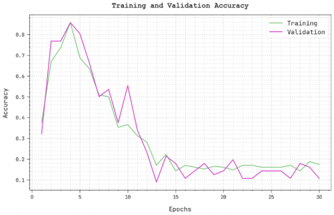
The training accuracy (TRA) and validation accuracy (VLA) developed using the DMODL-SC technique under test database are demonstrated in Figure 7. The simulated result inferred that the DMODL-SC approach has been able maximal value of TRA and VLA. Especially the VLA seemed to be high than TRA.
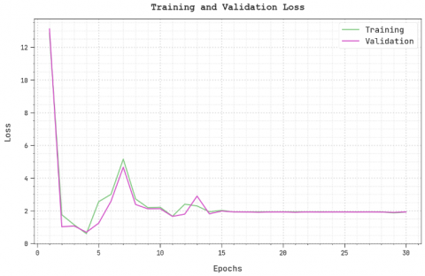
The training loss (TRL) and validation loss (VLL) achieved by the DMODL-SC methodology under test database are determined in Figure 8. The simulated result revealed that the DMODL-SC approach has acquired least values of TRL and VLL. Particularly, the VLL is lower than TRL.
A clear precision-recall (PR) inspection of the DMODL-SC technique under test database is portrayed in Figure 9. The figure indicated that the DMODL-SC system has resulted in improved values of PR values under all classes.
Figure 6. Average analysis of DMODL-SC system under 70:30 of TR/TS database
Figure 7. TRA and VLA analysis of DMODL-SC system
Figure 8. TRL and VLL analysis of DMODL-SC system
Figure 9. Precision-recall analysis of DMODL-SC system
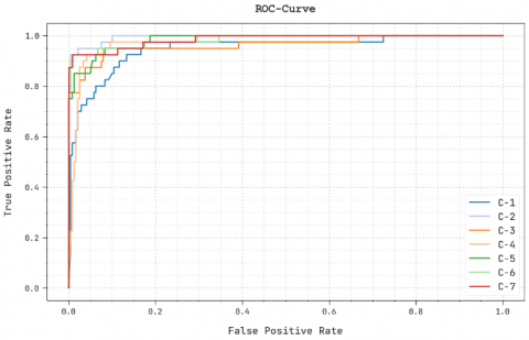
Figure 10. ROC curve analysis of DMODL-SC system
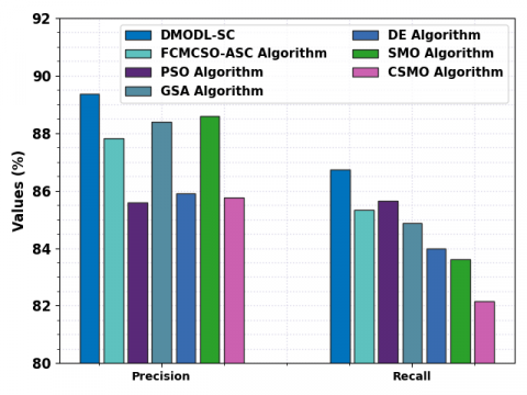
Figure 11. precn and recal analysis of DMODL-SC system with existing approaches
A brief ROC examination of the DMODL-SC approach under test database is illustrated in Figure 10. The results denoted the DMODL-SC method has displayed its capability in classifying different classes under test database.
Table 4 provides a comparative soil classification results of the DMODL-SC model and existing models [21]. Figure 11 reports a comparative precn and recal examination of the DMODL-SC model and existing models. The figure implied that the PSO, DE, and CSMO models have shown reduced values of precn and recal. Next, the FCMCSO-ASC model has attained slightly increased precn and recal of 87.81% and 85.32% respectively. Although the GSA and SMO models have obtained reasonable precn and recal values, the presented DMODL-SC model outperformed the existing models with maximum precn and recal values of 89.37% and 86.73% respectively.
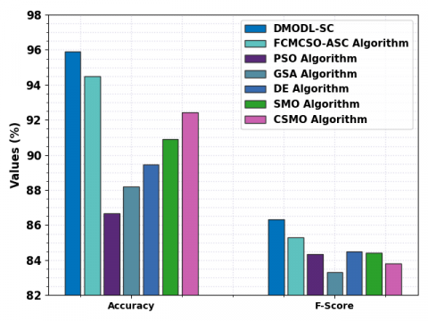
Figure 12. accuy and Fscore analysis of DMODL-SC system with existing approaches
Table 4. Comparative analysis of DMODL-SC system with existing approaches
|
Methods |
Precision |
Recall |
Accuracy |
F-Score |
|
DMODL-SC |
89.37 |
86.73 |
95.92 |
86.32 |
|
FCMCSO-ASC algorithm |
87.81 |
85.32 |
94.48 |
85.31 |
|
PSO algorithm |
85.60 |
85.64 |
86.66 |
84.33 |
|
GSA algorithm |
88.39 |
84.86 |
88.20 |
83.29 |
|
DE algorithm |
85.89 |
83.99 |
89.47 |
84.51 |
|
SMO algorithm |
88.59 |
83.62 |
90.91 |
84.41 |
|
CSMO algorithm |
85.75 |
82.16 |
92.42 |
83.82 |
Figure 12 shows a comparative accuy and Fscore inspection of the DMODL-SC method and present approach. The figure shows that the PSO, DE, and CSMO techniques have demonstrated reduced values of accuy and Fscore. Then, the FCMCSO-ASC technique accomplished slightly improved accuy and Fscore of 94.48% and 85.31% correspondingly.
Even though the GSA and SMO methods have acquired reasonable accuy and Fscore values, the presented DMODL-SC approach outperformed the existing models with maximum accuy and Fscore values of 95.92% and 86.32% correspondingly. These results show the enhanced soil classification results of the DMODL-SC model.
In this article, a novel DMODL-SC model was established for automated soil classification. The presented DMODL-SC technique majorly recognizes different kinds of soil using CV and DL models. In the presented DMODL-SC technique, the BF technique is used for noise removal process. In addition, the presented DMODL-SC technique employed the CapsNet model for feature extraction process. Moreover, DMO with DAE is exploited for the identification and classification of soil. To demonstrate the enhanced performance of the projected DMODL-SC system, an extensive range of experiments were performed. The comparison study reported the improvised soil classification performance of the DMODL-SC technique over other approaches with maximum accuracy of 95.92%. The DMODL-SC model offers enhanced performance and adaptability, addressing the challenges in noisy soil image data while optimizing hyperparameters. In upcoming work, the model's potential can be further discovered in real time agricultural and environmental situations like land management, accuracy agriculture and soil quality valuation. In addition, increasing model's abilities to handle large-scale, multi-modal data bases and integrating interpretability features for area professionals will be vital guidelines for upcoming study, safeguarding sustained development and applied value of DMODL-SC in soil organization and related fields.
[1] Srivastava, P., Shukla, A., Bansal, A. (2021). A comprehensive review on soil classification using deep learning and computer vision techniques. Multimedia Tools and Applications, 80: 14887-14914. https://doi.org/10.1007/s11042-021-10544-5
[2] Azizi, A., Gilandeh, Y.A., Mesri-Gundoshmian, T., Saleh-Bigdeli, A.A., Moghaddam, H.A. (2020). Classification of soil aggregates: a novel approach based on deep learning. Soil and Tillage Research, 199: 104586. https://doi.org/10.1016/j.still.2020.104586
[3] Inazumi, S., Intui, S., Jotisankasa, A., Chaiprakaikeow, S., Kojima, K. (2020). Artificial intelligence system for supporting soil classification. Results in Engineering, 8: 100188. https://doi.org/10.1016/j.rineng.2020.100188
[4] Zhang, Y.G., Xie, Y.L., Zhang, Y., Qiu, J.B., Wu, S.X. (2021). The adoption of deep neural network (DNN) to the prediction of soil liquefaction based on shear wave velocity. Bulletin of Engineering Geology and the Environment, 80: 5053-5060. https://doi.org/10.1007/s10064-021-02250-1
[5] Devine, S.M., Steenwerth, K.L., O'Geen, A.T. (2021). A regional soil classification framework to improve soil health diagnosis and management. Soil Science Society of America Journal, 85(2): 361-378. https://doi.org/10.1002/saj2.20200
[6] Moon, J.S., Kim, C.H., Kim, Y.S. (2022). Soil classification from piezocone penetration test using fuzzy clustering and neuro-fuzzy theory. Applied Sciences, 12(8): 4023. https://doi.org/10.3390/app12084023
[7] Hu, Y., Wang, Y. (2020). Probabilistic soil classification and stratification in a vertical cross-section from limited cone penetration tests using random field and Monte Carlo simulation. Computers and Geotechnics, 124: 103634. https://doi.org/10.1016/j.compgeo.2020.103634
[8] Li, X.Y., Fan, P.P., Li, Z.M., Chen, G.Y., Qiu, H.M., Hou, G.L. (2021). Soil classification based on deep learning algorithm and visible near-infrared spectroscopy. Journal of Spectroscopy, 2021: 1-11. https://doi.org/10.1155/2021/1508267
[9] Teng, H.F., Rossel, R.A.V., Shi, Z., Behrens, T. (2018). Updating a national soil classification with spectroscopic predictions and digital soil mapping. Catena, 164: 125-134. https://doi.org/10.1016/j.catena.2018.01.015
[10] Kyebogola, S., Burras, L.C., Miller, B.A., Semalulu, O., Yost, R.S., Tenywa, M.M., Lenssen, A.W., Kyomuhendo, P., Smith, C., Luswata, C.K. Majaliwa, M.J.G., Goettsch, L., Colfer, C.J.P., Mazur, R.E. (2020). Comparing uganda's indigenous soil classification system with world reference base and USDA soil taxonomy to predict soil productivity. Geoderma Regional, 22: e00296. https://doi.org/10.1016/j.geodrs.2020.e00296
[11] Xiao, T., Zou, H.F., Yin, K.S., Du, Y., Zhang, L.M. (2021). Machine learning-enhanced soil classification by integrating borehole and CPTU data with noise filtering. Bulletin of Engineering Geology and the Environment, 80: 9157-9171. https://doi.org/10.1007/s10064-021-02478-x
[12] Shivhare, S., Cecil, K. (2021). Automatic soil classification by using gabor wavelet & support vector machine in digital image processing. In 2021 Third International Conference on Inventive Research in Computing Applications (ICIRCA), IEEE, 1738-1743. https://doi.org/10.1109/ICIRCA51532.2021.9544897
[13] Yu, Y., Xu, T.F., Shen, Z.Y., Zhang, Y.H., Wang, X. (2019). Compressive spectral imaging system for soil classification with three-dimensional convolutional neural network. Optics Express, 27(16): 23029-23048. https://doi.org/10.1364/OE.27.023029
[14] Aditya Shastry, K., Sanjay, H.A. (2019). Cloud-based agricultural framework for soil classification and crop yield prediction as a service. In Emerging Research in Computing, Information, Communication and Applications (ERCICA), Springer Singapore, 1: 685-696. https://doi.org/10.1007/978-981-13-5953-8_56
[15] Bouayad, D., Baroth, J., Dano, C. (2021). Gaussian mixture model based soil classification using multiple cone penetration tests. In IOP Conference Series: Earth and Environmental Science, IOP Publishing, 696(1): 012034. https://doi.org/10.1088/1755-1315/696/1/012034
[16] Radhika, K., Madhavi Latha, D. (2019). Machine learning model for automation of soil texture classification. Indian Journal of Agricultural Research, 53(1): 78-82. https://doi.org/10.18805/IJARe.A-5053
[17] Naveen, P., Sivakumar, P. (2021). Adaptive morphological and bilateral filtering with ensemble convolutional neural network for pose-invariant face recognition. Journal of Ambient Intelligence and Humanized Computing, 12: 10023-10033. https://doi.org/10.1007/s12652-020-02753-x
[18] Deepika, J., Rajan, C., Senthil, T. (2022). Improved CAPSNET model with modified loss function for medical image. Signal, Image and Video Processing, 16(8): 2269-2277. https://doi.org/10.1007/s11760-022-02192-5
[19] Meng, Z., Zhan, X.Y., Li, J., Pan, Z.Z. (2018). An enhancement denoising autoencoder for rolling bearing fault diagnosis. Measurement, 130: 448-454. https://doi.org/10.1016/j.measurement.2018.08.010
[20] Agushaka, J.O., Ezugwu, A.E., Abualigah, L. (2022). Dwarf mongoose optimization algorithm. Computer Methods in Applied Mechanics and Engineering, 391: 114570. https://doi.org/10.1016/j.cma.2022.114570
[21] Dutta, A.K., Albagory, Y., Al Faraj, M., Alsanea, M., Sait, A.R.W. (2023). Cat swarm with fuzzy cognitive maps for automated soil classification. Computer Systems Science & Engineering, 44(2): 1419-1432. https://doi.org/10.32604/csse.2023.027377