Abd El Mouméne Zerari*![]() | Nadia Azri
| Nadia Azri ![]() | Mohamed Nadjib Meadi
| Mohamed Nadjib Meadi ![]() | Mohamed Chaouki Babahenini
| Mohamed Chaouki Babahenini ![]()
© 2023 IIETA. This article is published by IIETA and is licensed under the CC BY 4.0 license (http://creativecommons.org/licenses/by/4.0/).
OPEN ACCESS
A crucial element that sets apart realistic images from counterfeit ones is the inclusion of soft shadows. Despite the numerous techniques proposed to achieve this effect, the expense associated with computing precise soft shadows per pixel means that they continue to be excessively costly, primarily due to the necessity of a substantial number of rendering passes. To replicate accurate soft shadows in real-time applications, it is necessary to divide the area light into multiple samples and create a distinct shadow map for each of these samples. Subsequently, these shadow maps are merged to attain the intended visual effect. To obtain correct soft shadows, many shadow maps must be created, making the calculation procedure time-consuming. We suggest an innovative approach aimed at decreasing the rendering time necessary for real-time rendering while generating exact soft shadows. We advocate for reducing the number of samples in area lights to optimize soft shadow generation. Our technique is inspired by the Cascaded Shadow Maps (CSM) method use several shadow maps at different resolutions. It enables us to decrease area light source samples on specified areas of the waterfall view frustums. Furthermore, we develop a GPU-based filter with different kernels for each subfrusta to remove artifacts. In our experiments, our approach reduced rendering times until 51%. This method effectively removes artifacts, softens the resulting soft shadows, and decreases the computation time. The outcomes demonstrate that our strategy enhances efficiency by producing real-time soft shadows of exceptional quality at a faster pace than existing methods.
screen space, soft shadows, cascaded shadow maps, filtering, GPU
The purpose of this article is to propose a method for generating real-time soft shadows. The main objective is to enhance computational efficiency, minimize the required calculation time, and uphold image quality. We introduce a novel strategy that utilizes cascaded soft shadow maps, along with multiple Percentage-Closer Filtering kernels. This amalgamation allows for the generation of precise, top-notch real-time rendering of soft shadows, while significantly decreasing the overall rendering time.
Shadows play a crucial role in virtual worlds, given that they offer information about object geometry and position while also enhancing realism. Hard shadows, usually created by a point or directing light sources, can appear artificial and lack authenticity [1]. Conversely, soft shadows exhibit a degree of softness, providing a more natural and visually appealing appearance. However, accurately and efficiently calculating soft shadows proves to be a challenging and time-consuming task due to the large number of rendering passes [2]. Area light provides soft shadows, as opposed to point sources, which are responsible for hard shadows.
Creating shadows in rendering entails dealing with visibility issues between points and surfaces. To generate their effect, hard shadows only require determining the assessment of visibility between two specific points for every individual pixel. The challenges intensify in real-time applications where computational resources are limited, as techniques for global illumination that provide accurate results are computationally expensive. To address this, approximation methods are commonly used, but even these can be demanding. Frequently employed techniques for applications in real-time encompass shadow mapping [3] and shadow volume algorithms [4]. Shadow maps are 2D depth maps used to determine the visibility of light from the viewpoint of a camera or light source. They allow for scene geometry flexibility but is susceptible to perspective aliasing. To overcome this challenge, a solution known as Cascaded Shadow Maps [5] has been devised. CSMs aim to enhance depth texture resolution in the proximity of the viewer and reduce resolution in distant regions by partitioning the camera field of view and creating a depth map for each segment.
Nonetheless, generating realistic soft shadows necessitates the creation of a considerable number of shadow maps, resulting in increased computation time. In real-time applications, it becomes crucial to limit the quantity of samples. To address this, various methods [6-8] have been devised to reduce the number of samples utilized in the production of soft shadows.
Schwarzler et al. [7] proposed an innovative technique titled Fast Accurate Soft Shadows with Adaptive Light Source Sampling (FASSALSS) for area light source sampling called adaptive light source subdivision. The method begins with just a few samples and dynamically generates more sampling points as needed. Despite its potential benefits, this approach faces challenges in real-time applications due to the significant and rapid changes in penumbra area sizes and varying sample requirements within short timeframes. Consequently, its feasibility for real-time applications is limited.
We validate our method across various popular techniques, including Hatam [6], FASSALSS [7], and PCSS [9], demonstrating improved visual results in significantly reduced computation time.
Specifically, our primary contributions include: An open and interactive system designed for precise shadow rendering, suitable for use in 3D environments. Introduce a novel method for generating cascaded soft shadows that results in a substantial decrease in the required number of 3D scene renderings. The implementation of a precise and effective shadow method.
This paper is organized as follows: Section 2 examines existing methods that are relevant to our approach. Section 3 provides the required context, including formulas and methodologies. Section 4 offers a comprehensive insight into our real-time rendering technique and elucidates the procedure for generating soft shadows. This entails the utilization of various PCF kernels and distinct cascading shadow map resolutions. Section 5 displays the results, and offers a comparison of the various approaches. Lastly, we wrap up the study in Section 6, providing conclusions and outlining potential avenues for future research.
The methods for creating soft shadows can be categorized into three main types.
Firstly, methods that rely on filtering to blur the harsh shadow boundaries. Annen et al. [10] introduced a real-time soft shadow technique based on convolution, enabling constant-time processing and handling multiple area light sources. While sacrificing some precision for speed, this method produces believable results. Similarly, Chan and Durand [11] proposed a real-time shadow rendering technique using smooths, enhancing the shadow map approach for soft shadow approximation without intensive area light sampling. However, the generated shadows may have inaccuracies. Various efforts have been made to solve concerns such as aliasing. To soften strong shadow edges, Reeves et al. [12] developed the Percentage Closer Filtering (PCF) approach. PCF compares the depth in the shadow map to neighbouring pixels and estimates shadow intensity based on the percentage of successful shadow tests. While PCF eliminates aliasing artifacts and softens shadows, the size of the filter mask is fixed. As an upgrade to PCF, Randima [9] presented the Percentage Closer Soft Shadows (PCSS) approach. In the shadow map, PCSS adds extra blocker searches, allowing change of the filter kernel based on the interaction between light, blocker, and receptor. Several pre-filtering approaches have been developed [13, 14] to alleviate the high computational cost of PCF, allowing for real-time frame rates.
Secondly, approaches that depend on cascading techniques. Engel [5] presents a method called Cascaded Shadow Maps for rendering realistic shadows. By dividing the camera view cone into cascades and generating independent shadow maps for each, it overcomes the constraints of classical shadow mapping. These cascades span certain distance ranges, allowing for different shadow map resolutions for greater precision and the creation of high-quality shadows in modern real-time rendering processes. CSM enhances shadow quality, optimizes resource utilization, and keeps real-time performance constant. However, issues like waterfall limit artifacts and dynamic waterfall changes necessitate careful tailoring. Another option is to divide the viewing frustum into lesser dimension portions and produce a shadow map for every. The leading edge can be used to divide the frustumor via z-splitting, which involves cutting it along the view axis [15]. Techniques for reparameterization optimize sample placements for each face. Furthermore, "Backprojection" methods [16-19] have been described, which discretize the scene in a shadow map and calculate obscuration based on visibility parameters in screen space. While these algorithms provide more precise shading than PCF, shadow blockers that overlap are a constant problem for them, resulting in the projection of an enormous amount of texels from the shadow map, it impairs performance.
Thirdly, techniques that rely on sampling strategies. The methods employs a weighted sum of a collection of hard shadow samples captured from an area or volume light source [4]. Several studies have explored simplified geometries [20, 21] or light representations [22] to achieve real-time shadow rendering. Researchers have proposed various methods [23-25] to speed up this sampling process through density and weight adjustments. Ali et al. [6] proposed a real-time soft shadow approach titled Soft bilateral filtering shadows using multiple image-based algorithms (SBFS) that relied on bilateral filtering. Multiple light sampling point arrays are used, also softens the penumbra region in image space using bilateral filtering. This method minimizes the number of shadow maps, which results in better performance and outstanding effects. Recent works [26-28] try to generate realistic and rapid soft shadows but fall short in terms of physical correctness. To produce accurate soft shadows, create a shadow map for each sample after sampling the local light source, with the accumulated results producing accurate soft shadows. This method is time-consuming because of the enormous number of light source samples needed. Heckbert and Herf [29] suggested combining shadow maps for each receiver using an accumulation buffer to improve computation time by minimizing sample count. They also introduced precomputation techniques, however the computing complexity grows quadratically as the amount of receptors and light source samples increases. Agrawala et al. [22] improved on this approach by using a scene-wide single-layer attenuation map and combining it with depth image coherence-based ray tracing to achieve interactive rendering rates. St-Amour et al. [30] combined visibility information into numerous shadow maps for displaying soft shadows with the use of a previously computed compressed 3D visibility structure. Scherzer et al. [31] leveraged temporal coherence by sampling a light source across many frames, demonstrating examples where correct findings are obtained despite the obstacles posed by fast-moving objects. Schwarzler et al. [7] demonstrated a revolutionary real-time method for creating proper soft shadows. Their method selects sample locations by focusing on gentle shadows cast by region light sources and using a subdivision with adaptive light sources. Initially, a few bright-area samples are acquired, and the difference is tested using Hardware Occlusion Queries (HOQ) [32]. When necessary, additional sampling points are introduced, leading to a reduction in the quantity of light source samples. This enhancement enhances realism while also minimizing computational time. The usage of HOQ, on the other hand, causes rendering latency owing to GPU-CPU interactions.
In this article, we draw inspiration from the PCF approach but take a unique approach by utilizing multi-kernel PCF filtering. Similarly, we are inspired by the cascaded soft shadow mapping technique but implement it differently by employing cascading soft shadow mapping.
The aim of this study is to present a novel method for producing precise soft shadows. This is accomplished by combining multi-kernel PCF filtering and cascaded soft shadow mapping, with the primary goal of increasing speed while preserving good visual quality. Our contribution guarantees that he samples from the most pertinent area of light are selected, resulting in realistic and excellent delicate shadows suited for rendering in real-time. We compare our technique to cutting-edge rendering methods [6, 7, 9], illustrating its efficient equilibrium between computational time as well as visual quality.
3.1 Calculates soft shadows based on area light source
This section presents the soft shadow formula, derived according to Kajiya rendering formula, along with a proposed approach for simulating soft shadows using area light sources through the subdivision technique.
When rendering shadows, three distinct regions are considered: the umbra, where the light is entirely blocked, the penumbra area, where the light is partially visible, and the illuminated area, which receives full illumination from the light source.
Eisemann et al. [33] in their work proposes a formula for soft shadow area light source sampling:
$\textit{Soft}$_$\textit{Shadow}(p) = \frac{\mathbf{1}}{|\boldsymbol{S}|} \int_S V(p, s) \, ds$ (1)
where, Soft_Shadow(p) is the soft shadow value at point p, S constitutes a set comprising s points that define the light's surface, these points will be denoted as light samples. The visibility function, denoted as V(p,s), is then defined as follows:
$V(p, s)=\left\{\begin{array}{l}1 \text { if } p \text { and } s \text { exhibit mutual visibility } \\ 0 \text { else }\end{array}\right.$ (2)
For real-time rendering, performing the integration outlined in Eq. (1) for every point on the area light source S proves to be prohibitively cost. To approximate this integration, our focus lies on stochastic techniques for indirect illumination, specifically of the Monte-Carlo variety [34]. Monte Carlo sampling is used to estimate the value of an integral.
It is based on the principles of random sampling. The integral for Eq. (1) is estimated by finding the function's weighted average values at a set of randomly picked points:
$V_S(p) \approx \sum_{i=1}^N w_i V\left(p, s_i\right)$ (3)
The visibility assessment, denoted as V(p, si), is a result of a rigorous shadow visibility evaluation executed by shadow map i from the perspective of light si at point p. Only point light samples si carrying respective weights wi contribute to visibility determination, where $\sum_{i=1}^N w_i=1$.
The visibility factor, denoted as VS(p), is approximated through a weighted mean of visibility samples. This estimation is performed using the Monte-Carlo estimator, this accuracy improves with a rise in the number of samples [35].
Sampling the area light using N point lights enables the creation of a soft shadow effect. The soft shadow is then estimated using the shadow map ratio, denoted as SN.
$S_N=\frac{1}{N} \sum_{i=1}^N V\left(p, s_i\right)$ (4)
Given a square-shaped light source with an area S. Then we sample the light from the area using N light points, then for each light point we generate a shadow map. In a rendering pass we evaluate the visibility V(p, si) which is the result of a rigorous evaluation of the visibility of shadows performed by shadow map i from the point of view of light if at point p.
3.2 Shadow maps
Shadow mapping algorithms [3] involve two stages. Initially, the scene is rendered from the light position, followed by a recreation of the entire image from the camera's perspective. Pixels visible in the second rendering but not in the first indicate shadowed areas, while the remaining pixels represent illuminated regions. Its basic functioning principles are as follows:
Shadow Map Generation:
(1) Shadow Map Generation:
·Create a depth map (shadow map) by rendering the scene from the perspective of the light source.
·The depth map keeps track of the distance between the light source and the objects in the picture.
(2) Shadow Test:
·Create a depth map (shadow map) by rendering the scene from the perspective of the light source.
·The depth map keeps track of the distance between the light source and the objects in the image.
(3) Shadowing Algorithm:
·Sample the shadow map during the final scene rendering to calculate a shadow factor (0 for shadowed, 1 for bright) for each pixel.
·To simulate shadows, modify the final lighting calculations with the shadow factor.
Shadow maps prove advantageous in generating soft shadows and mitigating aliasing, with numerous algorithms seamlessly integrating soft edges.
This section introduces our novel method to generate soft shadows from a surface light source. Our main objective is to replicate authentic soft shadows achieved by accumulating multiple shadow maps. Each shadow map represents a sample simulating a point light source, which collectively contributes to the creation of the desired soft shadow effect. By employing this approach, we can achieve accurate soft shadows, greatly enhancing the realism of rendered scenes.
Our primary contribution lies in the utilization of shadow maps with variable resolutions and the application of PCF filters with different kernels. We divide the frustum into several subfrusta and employ a shadow map featuring multiple depth values for each light point. Additionally, we sample the surface light source for each subfrusta using different kernel sizes. As a result, we employ PCF filters with varying kernel sizes. To control the subdivision of the light area, we rely on HOQ to determine when to discontinue the subdivision process.
The suggested method is motivated by the works:
·Wolfgang Engel method [5], which involves partitioning the field of view into sections with varying texture resolutions.
·The FASSALSS technique [7], which is utilized for subdividing area lights and optimizing the stopping test.
·The utilization of texture arrays enables us to create as many as 512 textures in each rendering pass.
·PCF technique is used to filter the edges of shadows to eliminate aliasing.
However, our approach involves subdividing the light using a limited set of samples. We present a novel technique that we've named Cascaded Soft Shadow Maps, utilizing PCF filters with various kernels. This strategy enables us to augment the sample count in proximity to the viewer while concurrently diminishing the samples as the distance increases. To achieve this, we partition the camera view separately and construct depth maps for the point light samples in each partition.
4.1 Detailed explanation of our method
In this part, we introduce our novel idea for each cascade, which involves utilizing shadow maps associated with individual point light sources and employing multiple PCF filters to merge the cascaded shadow maps.
By partitioning the camera view frustum, we achieve higher-resolution depth textures near the viewer, using a unique version of the CSM technique. This division facilitates the creation of depth maps for point light samples in each partition, thereby improving quality and decreasing computation time.
The proposed technique is implemented in the following steps: Firstly, for each cascade, we partition the area light into N (see Formula 6) individual point light sources. Subsequently, we generate the respective shadow maps by rendering the scene from the viewpoint of each point light source. Next, we further divide the visual frustum into several subfrusta (splits). During a future rendering phase, we compute the soft shadow value corresponding to every subfrustum (cascade). To reduce the number of render passes, we use a PCF filter with different kernels to soften the generated shadows. Finally, we illuminate the area using a shading model.
Algorithm of our technique
1: 3D scene modeling.
2: First render pass:
3: Partition frustum into subfrusta; // see Formula (7)
4: For each subfrusta do
5: If this subfrusta contains object then
6: Taking a sample of the light; // see Sect. 4.1.1- B
7: For each point light do
8: Generate a shadow map; // see Sect. 4.1.1- D
9: Render of the scene from the point of view of this point light;
10: Save this shadow map in texture array;
11: End For
12: End If
13: End For
14: Final render pass
15: For each subfrusta do
16: Determine the kernel sizes for each subfrusta; // see Sect. 4.1.2 - E
17: For shadow map do
18: Do the depth test; // see Sect. 4.1.2
19: Use filtering with PCF;
20: Screen display;
21: End For
22: End For
4.1.1 First render pass
A. Partition frustum into subfrusta
The act of forming subfrusta is known as partitioning the frustum (see Figure 1). The truncated cone is divided into intervals along the Z-axis, covering from 0% to 100%. Each interval, with respect to the Z-axis, defines a near plane (0%) and a far plane (100%).
Figure 1. Subdivision of a square area light with 25, 9 and 4 samples
To optimize shadow rendering, the view frustum is divided into three cascades: near, middle, and far. Each cascade is rendered into its dedicated shadow maps. The depth sampling from the shadow maps is governed by the viewer's distance, while the shadow algorithm remains unchanged. A large number of samples are employed in the near cascade to build high-resolution shadow maps for close objects, assuring high-quality shadows. A medium number of samples are used in the middle cascade to generate medium-resolution shadow maps, while a small number of samples are used in the far cascade to generate low-resolution shadow maps for distant objects, lowering computing overhead for objects far from the camera.
Inspired by the research of Zhang et al. [15], we determined the z-value distance between these sub-frustums as a means to divide the field of view:
$Z_i=\frac{n(f / n)^{i / m}+n+(f-n)^{i / m}}{2}, \forall 0 \leq i \leq m$ (5)
where, m stands for the number of separated sections sections (1≤i≤m-1), n and f are the near and distant planes of the view frustum, and Z0=n+0.5 and Zm=f. Zi stands for the depth of the ith sections plane in view space.
B. Taking a sample of the light
This section presents our method for sampling surface light, employing a uniform division of the square region light source. Initially, we divide the area light source into four point lights, each placed at a corner of the square. Eq. (6) guides the generation of additional point lights as needed for further subdivisions of this area light.
$N=k^2$ (6)
After generating the initial sample points, it's important to check for the presence of artifacts. If any artifacts are detected, the light source needs to undergo further subdivision, accompanied by the formation of shadow map depths (refer to Eq. 7).
To rapidly assess the necessity for subdivision, we use HOQ [32], a technique commonly utilized to gauge visibility based on screen pixel count. By discarding fragments with sufficient subdivision levels, we can efficiently tally the remaining fragments. If any pixel is output, it indicates the area light source requires further refinement in this frame.
C. Sampling of the area light
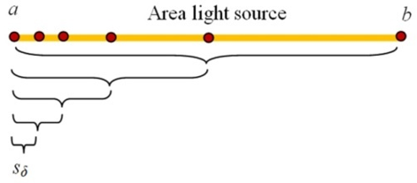
We apply a conventional subdivision method to handle the edges of the area light. The partitioning of the boundary [a, b] of the region light source constitutes a set denoted as ν=(x0, x2, x3, ….., xu) of u+1 points in [a,b], Considering a real number u ∈ $\mathbb{R}$, satisfying the condition: a=x0<x1<x2………<xf<xf+1<…<xu=b. This stems from the partitioning of the interval [a, b] into u sub-intervals. Consequently, the standard step for subdivision is as follows:
$\forall \delta \in[0, u], x_\delta=a+\delta \times \frac{(b-a)}{u}$ (7)
Here, δ represents a variable determining the extent of a section that originates from the distance between two points, denoted as a and b (referring to the dimensions of the light source, with a<b).
On the other hand, the quantity of samples generated through conventional subdivision can be expressed as follows: N= (2δ+1)2, where δ represents the level of subdivision.
Figure 2. Subdivide area light source edge
Figure 2 illustrates the regular subdivision technique employed in our method for computing the minimal distance denoted as xδ between two light samples. This process is iterated until the distance becomes smaller than or equal to the threshold specified by the HOQ.
D. Generate a shadow map
We begin by selecting the appropriate resolution for the shadow map that matches the requirements of this subfrusta. From the perspective of the current point light source, we generate a shadow map specifically for this subfrusta. Our process starts with a meticulous initialization phase, where we set all the essential parameters.
It should be noted that employing numerous shadow maps can present challenges due to technical limitations. To overcome this issue, we leverage Texture Arrays, introduced through graphics APIs, which streamline the management of multiple textures in practical applications. These Texture Arrays empower the shader to handle up to 512 textures with consistent sizes and formats. This feature offers significant benefits to our tasks, enabling us to seamlessly integrate numerous shadow maps within a unified shader, enhancing overall efficiency. Specifically, we use the Texture Array composed of individual elements, each housing a depth shadow map. The utilization of this texture array empowers us to effectively handle a substantial quantity of uniform-sized and formatted shadow maps, which improves the overall efficiency and performance of our rendering strategy.
After we've created the shadow map for the specific subfrusta, we'll save and store it in the texture array. By properly maintaining many shadow maps, this texture array serves a critical role in optimising our rendering process.
4.1.2 Final render pass
Within this section, our central emphasis lies in the creation of soft shadows through the utilization of cascading shadow maps. This is assessable in a solitary, ultimate illumination rendering pass for all the generated shadow maps, akin to the secondary rendering pass found in the conventional shadow mapping algorithm.
We begin by rendering a scene pass from the camera's perspective and retrieving the elements from the texture array for each subfrusta. For every vertex, we conduct N (see Formula 6) shadow tests for each point light source of the area light source. Subsequently, the outcomes are averaged to ascertain the magnitude that symbolizes the proportion of shadows assigned to the central pixel. This process ensures the realistic generation of soft shadows in our rendering technique.
A. Shadow map information evaluation
This step is performed after getting all of the necessary shadow maps. We explore and fix issues that may develop as a result of varying subdivision depths and the extensive sampling of depth textures.
B. Weight allocation for shadow maps
We use weights depending on subdivision areas to efficiently manage the sampling locations. Individual samples with smaller weights contribute less to the blackness of the penumbra in regions with more subdivisions than those with larger weights.
The computation of weights allocated to the ith shadow map pertaining to an area light source is carried out in the subsequent manner: $w_i=1 / k^2$, with k2 representing the quantity of samples, it is ensured that the cumulative sum of all weights amounts to 1.
Otherwise, the weights must be normalized to ensure that the final collected shadow values are between 0 (completely lighted) and 1 (fully shadowed).
C. Compute soft shadows
In the shadow mapping procedure, the shadow map is assessed in a second pass from the perspective of the camera, using data from the previous pass for shadow computation. This step aims to determine soft shadows. To achieve this, the back-projection of every pixel is performed within the pixel shader to the frustum of every point light, and the depth of that specific pixel is compared from the light's perspective.
The result is a binary value (0 or 1), signifying whether the pixel is under shadow concerning a specific point light source i. These results are then scaled by their respective weights, aggregated, and used to compute the occlusion percentage. This computation facilitates the rendering of soft shadows within the displayed scene.
D. Determine the kernel sizes that are appropriate for each subfrusta
Due to the high sample density needed for smooth rendering, producing realistic soft shadows utilizing multiple shadow maps for each light source can place a significant computational load on the system. Noticeable banding artifacts can occur when only a few shadow maps are used.
The resolution of the shadow map plays a crucial role in mitigating the problem of aliasing. Shadow maps with low resolution have jagged and unsmooth edges, but higher resolutions effectively reduce aliasing. It's important to recognize that textures of higher quality come with a slightly higher cost compared to lower-resolution textures. To provide outstanding shadow quality and minimize aliasing artifacts. In our technique, we use three type of shadow map resolution, an appropriate resolution for each subfrusta.
Following the creation of shadow maps as detailed in the preceding section, we proceed to compute the kernel sizes for the PCF filter. In our approach, we utilize three distinct area light subdivisions (high, medium, and low) for each subfrustum. In the first subfrusta (see Figure 1), we use a 5×5-sample kernel, resulting in a high-resolution kernel for each shadow map. We use a medium-density kernel with 3×3 samples in the second subfrusta and a low-density kernel with 2×2 samples in the third subfrusta.
The use of PCF filtering enhances the softness of shadow boundaries significantly, and modern graphics hardware can support 5×5, 3×3, and 2×2 kernel versions without sacrificing speed.
E. Screen display
To imbue our scene with a sense of realism, we must account for the interplay of light and objects within the virtual environment. To accomplish this, we use the well-known Phong shading model [35]. This model makes correct light interaction calculations possible, resulting in a visually compelling and lifelike portrayal of our virtual world.
In this section, we'll go over the implementation outcomes, comparing and contrasting various performance and visual quality metrics.
The OpenGL Shading Language Shading graphics 4.7 API is used to build the rendering method on a GPU. All performance measurements and findings described in this article were acquired on a PC equipped with an Intel(R) Core(TM) i7-7700K CPU @ 4.20GHz, Nvidia GeForce GTX 1070/PCIe/SSE2, and 32 GB RAM running a 64-bit version of Microsoft Windows 8.1.
As standard criteria for comparing outcomes, we used FPS (Frames Per Second) and image production time. We used the RMSE (Root Mean Square Error) statistic to assess the efficacy of the suggested technique [36]. In addition, we used the Structual Similarity Index Measure (SSIM) metric [37] to assess the contrast of rendering quality, focusing on the SSIM contrast component. We employed SSIM index maps to compare images, with white denoting SSIM = 1 (indicating identical images), black indicating SSIM = 0, and SSIM values within [-1, 0] mapped to colors between red and green. All the outcomes presented in this section were obtained at a resolution of 800×600.
We validate the outcomes of our research through both qualitative and quantitative assessments, using real-time scene images. The test scenes encompass a diverse array of objects, and their depiction can be found in the references [38-40].
We showcase the results obtained from our novel technique for rendering cascaded correct soft shadows. The method is based on sampling the region light source and partitioning the camera view frustum. This division improves shadow quality for close objects while shortening calculation time. We compare our generated images using this technique to images synthesised using FASSALSS [7], SBFS [6], PCSS [9] methods, and the reference image (Ground Truth). The reference image is calculated with 256 samples from an area light source, showing the ideal expected outcome that closely reflects reality.
When discussing our method with 16, 9, and 4 samples, it indicates the utilization of a corresponding number of shadow maps for each sub-frustum, spanning from the near to the far plane.
5.1 Visual assessment and comparison
In this section, we'll discuss the implementation's outcomes while comparing and evaluating a number of performance and visual quality criteria.
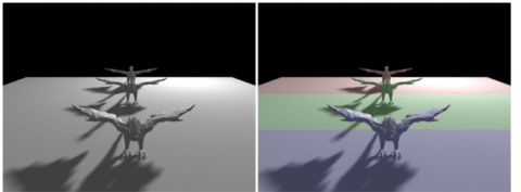
Figure 3 on the left shows an illustrative example made utilizing the suggested technique, involves dividing the field of view into three distinct sub-frustums, each with its own unique PCF filter, resulting in an FPS of 423. The picture on the right displays the distinct sub-frustums, each represented by a different color in its corresponding portion.
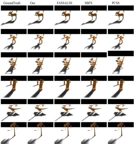
In Figure 4, we present a comparative analysis of our area light sampling technique against the methods proposed by [6, 7, 9], using various scenes. The images displayed on the left represent the ground truth, obtained by employing 256 samplings of area light, which serve as the reference for comparing the other images. The middle column on the left showcases outcomes achieved through our approach using 16, 9, and 4 shadow maps respectively. The middle column displays images created through FASSALSS approach [7] utilizing 25 shadow maps. Similarly, the middle-right column exhibits images produced using SBFS method [6], which also employs 25 shadow maps. Furthermore, the far-right column presents images generated by the PCSS approach [9] with the use of 16 shadow maps.
Figure 3. Frustum area split into three part
Figure 4. Selected qualitative results for various methods and scenes
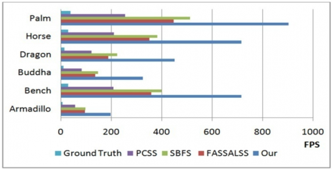
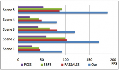
To analyze the performance, Figure 5 illustrates the frame rate results for images of Figure 4 generated by our technique using 16, 9 and 4 shadow maps, Ground Truth and the earlier approaches [6, 7, 9]. In Figure 5, we can observe the significantly enhanced interactive speeds of our innovative approach, which are approximately twice as fast as the methods presented in previous studies [6, 7]. These results demonstrate the superior performance and efficiency of our technique in generating soft shadows compared to earlier approaches, enabling real-time rendering of complex images. The significant speed improvement is attributed to the strategic implementation of view frustum subdivision and the use of different kernels per area.
Figure 5. The frame rate outcomes for our method, as well as for Ground Truth and other techniques [5, 6, 9], depending on different rendering scenes
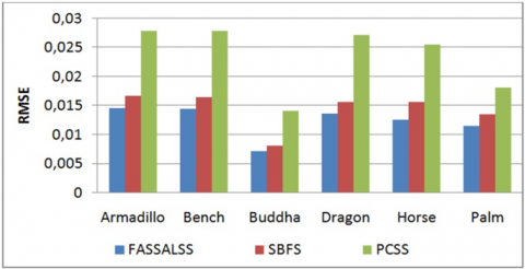
Figure 6 displays the RMSE values derived from the comparison of reference images created using our method, employing 16, 9, and 4 samples for each scene, and images produced by both methods [6, 7, 9] (identical pictures to those in Figure 4). The RMSE indicates that the SBFS [6] and FASSALSS [7] methods yields smaller values than the PCSS [9] for all scenes. As a result, the soft shadows produced by our technique are more similar to Ali’s method and FASSALSS method [7], making the shadows produced by our method correct, validating the accuracy of the shadows created through our approach.
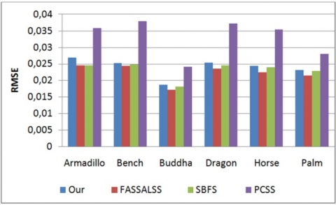
Figure 7 shows the Root Mean Square Error values calculated by comparing the ground truth image which uses 256 shadow maps, to images made using approaches from references [6, 7, 9], as well as our own method (depicted in Figure 4).
Figure 6. RMSE calculated between the reference images acquired with our technique employing 16, 9, and 4 samples and those generated by other approaches
Figure 7. An evaluation of RMSE values generated using 256 samples in conjunction with diverse methods
Figure 8. A visual contrast among various scenes using our proposed approach and SBFS method [6], as well as the RMSE and SSIM values
Figure 8 illustrates the qualitative results of diverse techniques employing area light sampling. The images in the left column showcase our suggested approach with 16, 9, and 4 samples. The middle column adjacent to it demonstrates images generated via SBFS method [6] employing 25 shadow maps. The middle column on the right displays the disparity between our approach and SBFS method [6], while the rightmost column presents SSIM index maps comparing the two. To validate our method's efficacy, we compute RMSE and SSIM values for distinct scenes (refer to Figure 8). The results show an RMSE less than 0.01, indicating essentially identical pictures, and SSIM values close to 1, showing significant similarity. Our soft shadows are crisp and precise. The disparity images and SSIM index maps reveal a notable resemblance between our approach, utilizing fewer area light samples, and SBFS technique [6]. The runtime in frames per second for both strategies demonstrates that our proposal outperforms SBFS method [6] by 44% to 51% without sacrificing visual quality.
Figure 9. Comparison of rendering outcomes for highly intricate scenes, with ground truth images with images generated using different methods
Figure 10. FPS of the images of Figure 9
In regard to Figure 9, we use the SSIM measure to validate the precision of our advanced technique for exceedingly complex scenes (see Figure 10). The images on the left portray intricate scenes in the sequence: ground truth with 256 samples, our technique with 16, 9, and 4 samples, and methods proposed by FASSALSS [7], SBFS [6], and PCSS [9] utilizing 16 samples. A comparison of SSIM values demonstrates that our strategy produces values that are closer to unity than the other approaches [6, 9]. Figure 11 depicts an evaluation of the frames per second (FPS) achieved by our technique in comparison to other methods. As a result, our technique produces more accurate images, and our results show that our suggested algorithm is both faster and more accurate.
As shown in all figures, our rendering system achieves a visual quality similar to FASSALSS method [7], utilizing a greater number of shadow maps than the alternative techniques. Moreover, Figures 4 and 8 serve to emphasize the heightened realism inherent in our approach when compared to SBFS method [6] and the PCSS technique [9]. This distinction can be attributed to our implementation of cascaded soft shadows and PCF with multiple kernels, a strategy incurring marginal computational overhead while retaining edge acuity. The accuracy of the soft shadows produced by our rendering system is substantiated by RMSE and SSIM values comparable to those of FASSALSS method [7].
Figure 11. SSIM values comparing the ground truth obtained from 256 shadow maps with alternative methods
The SBFS approach [6] and PCSS technique [9], on the other hand, provide larger RMSE values across scenes due to the smoothing effects of the filters, resulting in too smooth results. As a result, our strategy exceeds SBFS method [6] in terms of image quality while outperforming both methods in terms of runtime.
Performance
Our primary objective is to streamline the creation of precise soft shadows by optimizing the computational process, ultimately elevating the expected visual fidelity. This optimization in computation leads to a substantial improvement in rendering efficiency, resulting in a notable performance increase ranging from around 44% to 51% for each frame rendered.
We developed a novel technique for rendering exact soft shadows by merging the cascaded soft shadow map approach with PCF using multiple kernels. Our experimental application revealed the ability to generate soft shadows of equal quality to a produced using 256 shadow maps for the ground truth images while achieving interactive frame rates and even real-time rendering, ensuring quick outputs across a variety of situations, including complicated ones.
The fundamental feature of our technique is the use of cascaded soft shadows using shadow maps with varying resolutions within sub-frustums. Across frustum cascades, this technique optimizes render times and shadow map resolutions. Furthermore, using PCF with several kernels minimizes aliasing concerns in locations with vast penumbras.
Our approach has real-world applications and impact because of the advantages of our rendering system, which include greatly reduced computing time for soft shadow calculations, edge sharpness preservation, alias reduction, and the ability to consistently generate promising results. This technique has a lot of potential in a variety of interactive sectors, such as film production, architectural visualisation, virtual and augmented reality experiences, scientific visualisation, 3D gaming, and any application that requires accurate task lighting. When compared to existing methodologies, our research indisputably reveals improved rendering efficiency.
Due to the close closeness of a zone light to the ground, changes in the proportions of the penumbra zone can occur quickly, resulting in varied sample requirements. As a result, our rendering approach may not be optimal for real-time rendering, instead finding more practical uses in modeling and design contexts that require quick previews of precise soft shadows. Even using the most accessible shadow maps may not result in performance improvements in circumstances when both the proposed approach and a scene with substantial penumbra coexist. Furthermore, as the complexity of the scene escalates, the interactive capabilities of our algorithm experience a significant reduction.
Looking ahead, we propose potential improvements to significantly reduce calculation time, particularly in the shadow map algorithm's comparison step. This can be accomplished by minimizing occlusion queries in the penumbra zone by performing selective lookups on shadow maps for area light source samples, while handling shadows from a single point light source in the umbra zone. Such an approach would optimize filtering just in artifact-prone zones, thereby improving the overall performance of our accurate soft shadow rendering.
[1] Mamassian, P., Knill, D.C., Kersten, D. (1998). The perception of cast shadows. Trends in Cognitive Sciences, 2(8): 288-295. https://doi.org/10.1016/S1364-6613(98)01204-2
[2] Hasenfratz, J.M., Lapierre, M., Holzschuch, N., Sillion, F.X. (2003). A survey of real-time soft shadows algorithms. In Computer Graphics Forum, 22(4): 753-774. https://doi.org/10.1111/j.1467-8659.2003.00722.x
[3] Williams, L. (1978). Casting curved shadows on curved surfaces. In Proceedings of the 5th annual conference on Computer graphics and interactive techniques, pp. 270-274. https://doi.org/10.1145/800248.807402
[4] Crow, F.C. (1977). Shadow algorithms for computer graphics. ACM Siggraph Computer Graphics, 11(2): 242-248.https://doi.org/10.1145/965141.563901
[5] Engel, W. (2006). Shader X5: Advanced rendering techniques. Charles River Media, Inc..
[6] Ali, H.H., Kolivand, H., Sunar, M.S. (2017). Soft bilateral filtering shadows using multiple image-based algorithms. Multimedia Tools and Applications, 76: 2591-2608. https://doi.org/10.1007/s11042-016-3254-0
[7] Schwärzler, M., Mattausch, O., Scherzer, D., Wimmer, M. (2012). Fast accurate soft shadows with adaptive light source sampling. In: Proceedings of the 17th International Workshop on Vision, Modeling, and Visualization (VMV 2012), pp. 39-46. https://doi.org/10.2312/PE/VMV/VMV12/039-046
[8] Aszódi, B., Szirmay-Kalos, L. (2006). Real-time Soft shadows with shadow accumulation. In Eurographics(Short Presentations), pp. 53-56. http://dx.doi.org/10.2312/egs.20061026
[9] Randima, F. (2005). Percentage-closer soft shadows. In: Association for Computing Machinery, SIGGRAPH’05 Sketches, New York, NY, USA. https://doi.org/10.1145/1187112.1187153
[10] Annen, T., Dong, Z., Mertens, T., Bekaert, P., Seidel, H. P., Kautz, J. (2008). Real-time, all-frequency shadows in dynamic scenes. ACM Transactions on Graphics (TOG), 27(3): 1-8. https://doi.org/10.1145/1360612.1360633
[11] Chan, E., Durand, F. (2003). Rendering fake soft shadows with smoothies. In Rendering Techniques, pp. 208-218.
[12] Reeves, W.T., Salesin, D.H., Cook, R.L. (1987). Rendering antialiased shadows with depth maps. In Proceedings of the 14th annual conference on Computer graphics and interactive techniques, pp. 283-291.https://doi.org/10.1145/37401.37435
[13] Donnelly, W., Lauritzen, A. (2006). Variance shadow maps. In Proceedings of the 2006 symposium on Interactive 3D graphics and games, pp. 161-165.https://doi.org/10.1145/1111411.1111440
[14] Annen, T., Mertens, T., Bekaert, P., Seidel, H.P., Kautz, J. (2007). Convolution shadow maps. Rendering Techniques, 18: 51-60. https://doi.org/10.2312/EGWR/EGSR07/051-060
[15] Zhang, F., Sun, H., Xu, L., Lun, L.K. (2006). Parallel-split shadow maps for large-scale virtual environments. In Proceedings of the 2006 ACM international conference on Virtual reality continuum and its applications, pp. 311-318.https://doi.org/10.1145/1128923.1128975
[16] Mohankumar, S., Thimmaiah, G.M., Chikkaguddaiah, N., Gowda, V.B. (2021). MODFAT: Moving object detection by removing shadow based on fuzzy technique with an adaptive thresholding method. Revue d'Intelligence Artificielle, 35(2): 177-183. https://doi.org/10.18280/ria.350210
[17] Guennebaud, G., Barthe, L., Paulin, M. (2007). High-quality adaptive soft shadow mapping. In Computer Graphics Forum, 26(3): 525-533. https://doi.org/10.1111/j.1467-8659.2007.01075.x
[18] Vikruthi, S., Archana, M., Tanguturi, R.C. (2022). Shadow detection and elimination technique for vehicle detection. Revue d'Intelligence Artificielle, 36(5): 753-760. https://doi.org/10.18280/ria.360513
[19] Schwarz, M., Stamminger, M. (2007). Bitmask soft shadows. In Computer Graphics Forum, 26, (3): 515-524.https://doi.org/10.1111/j.1467-8659.2007.01074.x
[20] Fuchs, H., Goldfeather, J., Hultquist, J.P., Spach, S., Austin, J.D., Brooks Jr, F.P., Eyles, J.G., Poulton, J. (1985). Fast spheres, shadows, textures, transparencies, and imgage enhancements in pixel-planes. ACM Siggraph Computer Graphics, 19(3): 111-120. https://doi.org/10.1145/325165.325205
[21] Ren, Z., Wang, R., Snyder, J., Zhou, K., Liu, X., Sun, B., Sloan, P.P.G., Bao, H., Peng, Q.S., Guo, B. (2006). Real-time soft shadows in dynamic scenes using spherical harmonic exponentiation. In Acmsiggraph 2006 papers, pp. 977-986. https://doi.org/10.1145/1179352.1141982
[22] Agrawala, M., Ramamoorthi, R., Heirich, A., Moll, L. (2000). Efficient image-based methods for rendering soft shadows. In Proceedings of the 27th annual conference on Computer graphics and interactive techniques, pp. 375-384.https://doi.org/10.1145/344779.344954
[23] Franke, T.A. (2014). Delta voxel cone tracing. In 2014 IEEE International Symposium on Mixed and Augmented Reality (ISMAR), pp. 39-44. https://doi.org/10.1109/ISMAR.2014.6948407
[24] Mehta, S.U., Wang, B., Ramamoorthi, R. (2012). Axis-aligned filtering for interactive sampled soft shadows. ACM Transactions on Graphics (TOG), 31(6): 1-10. https://doi.org/10.1145/2366145.2366182
[25] Öztireli, A.C. (2016). Integration with stochastic point processes. ACM Transactions on Graphics (TOG), 35(5): 1-16. https://doi.org/10.1145/2932186
[26] Buades, J.M., Gumbau, J., Chover, M. (2016). Separable soft shadow mapping. The Visual Computer, 32(2): 167-178.https://doi.org/10.1007/s00371-015-1062-6
[27] Xu, Z., Li, B., Cai, X., Sun, H., Zhang, Y. (2015). Generate accurate soft shadows using complete occluder buffer. In 2015 14th International Conference on Computer-Aided Design and Computer Graphics (CAD/Graphics), pp. 97-104.https://doi.org/10.1109/CADGRAPHICS.2015.35
[28] Liktor, G., Spassov, S., Mückl, G., Dachsbacher, C. (2015). Stochastic soft shadow mapping. In Computer Graphics Forum, 34(4): 1-11.https://doi.org/10.1111/cgf.12673
[29] Heckbert, P.S., Herf, M. (1997). Simulating soft shadows with graphics hardware (p. 15213). Pittsburgh, PA: School of Computer Science, Carnegie Mellon University.
[30] St-Amour, J.F., Paquette, E., Poulin, P. (2005). Soft shadows from extended light sources with penumbra deep shadow maps. In Graphics Interface, pp. 105-112.https://dl.acm.org/doi/10.5555/1089508.1089526
[31] Scherzer, D., Schwärzler, M., Mattausch, O., Wimmer, M. (2009). Real-time soft shadows using temporal coherence. In Advances in Visual Computing: 5th International Symposium, ISVC 2009, Las Vegas, NV, USA, November 30-December 2, 2009. Proceedings, Part II 5, pp. 13-24.https://doi.org/10.1007/978-3-642-10520-3_2
[32] Bartz, D., Meißner, M., Hüttner, T. (1998). Extending graphics hardware for occlusion queries in OpenGL. In Proceedings of the ACM Siggraph/Eurographics workshop on Graphics hardware, pp. 97-103.http://dx.doi.org/10.2312/EGGH/EGGH98/097-103
[33] Eisemann, E., Schwarz, M., Assarsson, U., Wimmer, M. (2011). Real-time shadows. CRC Press.https://doi.org/10.1201/b11030
[34] Kajiya, J.T. (1986). The rendering equation. In Proceedings of the 13th annual conference on Computer graphics and interactive techniques, pp. 143-150.https://doi.org/10.1145/15922.15902
[35] Phong, B. (1975). Illumination for computer generated images. Communications of the ACM, 18(6): 311-317. https://dl.acm.org/doi/10.5555/906584.
[36] Willmott, C.J., Matsuura, K. (2005). Advantages of the mean absolute error (MAE) over the root mean square error (RMSE) in assessing average model performance. Climate Research, 30(1): 79-82.http://dx.doi.org/10.3354/cr030079
[37] Wang, Z., Bovik, A.C., Sheikh, H.R., Simoncelli, E.P. (2004). Image quality assessment: from error visibility to structural similarity. IEEE Transactions on Image Processing, 13(4): 600-612.https://doi.org/10.1109/TIP.2003.819861
[38] Stanford University. (1996). The Stanford 3D Scanning Repository. http://graphics.stanford.edu/data/3Dscanrep
[39] Morgan McGuire. (2017). Computer Graphics Archive. http://casualeffects.com/data/index.html
[40] Sketchfab community. (2012). To publish and find 3D content online, Paris, France. https://sketchfab.com/feed