Sumalatha Ganesh*![]() | Muthumani Nachimuthu
| Muthumani Nachimuthu![]()
© 2023 IIETA. This article is published by IIETA and is licensed under the CC BY 4.0 license (http://creativecommons.org/licenses/by/4.0/).
OPEN ACCESS
Gene Expression Microarray (GEM) data is biological data that contains valuable hidden information genes. The gene information extracted from variations of gene expression levels is utilized for disease detection and diagnosis, especially in cancer classification. Since GEM data contains a relatively large sample size with highly redundant and imbalanced data, the accuracy of the cancer classification result is lower. It is difficult to identify suitable features from large GEM datasets. Hence, in this paper, this model utilizes Grey Wolf Optimization (GWO) Model to select the features from the GEM data. Convolutional Neural Network with Long Short Time Memory (ConvLSTM) is developed by utilizing Deep Reinforcement Learning (DRL) to select the appropriate features and parameters for efficient cancer classification. The ConvLSTM model is used to convert low-level features into high-level ones by identifying distributed data representations. DRL optimizes ConvLSTM parameters iteratively which significantly impacts the overall learning process of this prediction model. In DRL, The Double Deep Q-Network (DDQN) model is introduced to minimize training-time overestimations of action values. Finally, the loss function is employed in the Neural Network (NN) of ConvLSTM for accurate cancer detection and diagnosis of cancer. The proposed model is termed Improved ConvLSTM using DDQN (ICL-DDQN). The ICL-DDQN-DDQN achieves accuracy of 92%, 91.67% and 92.22% for breast cancer, leukemia and lung cancer datasets which is 32.69%,57.16%, 23.89% higher than 1D-CNN; 21.06%, 43.18%, 16.89% higher than DL-DCGN; 15%, 28.33%, 10.18% higher than DL-SAE and 6.15%, 132.79%, 4.83% higher than DL-AAA on respective datasets. The proposed model effectively detects cancer at its earlier stage, reducing manual inspection and time for doctors and physicians, resulting in more effective treatment.
gene expression microarray, convolutional neural network, long short time memory, grey wolf optimization double deep Q-network
Cancer is defined by uncontrolled, abnormal cell development that may metastasis (spread to other regions of the body) [1]. Cancer is a potentially fatal illness that shortens people's lives; therefore, an accurate and timely diagnosis is critical. Early cancer identification requires a precise and reliable procedure, providing information about the patient's malignancy, enabling improved clinical decision-making and treatment [2]. Mutations in genes involved for cell proliferation and differentiation which cause normal cells to change into cancer cells.
DNA microarrays may be used to identify gene expression, which is a valuable tool for identifying, diagnosing, and forecasting the progression of cancer. Although a gene expression dataset may include hundreds of gene expressions, only a fraction of these genes is responsible for particular cancers [3]. Finding and isolating important genes and determining how they contribute to a disease is no easy feat [4]. Researchers gain access to a wealth of information through microarray GEM datasets, but it is difficult to find the relevant data without the right tools and methods. The abundance of raw gene expression data creates difficulties in analysis and computing. The feasible gene combination is a key factor in the best analytical models. This means that techniques are necessary for the successful analysis of GEM datasets for cancer detection. The main challenges is the GEM data is high dimensionality which is crucial in cancer detection and classification [5, 6].
In order to solve the dimensionality issues, feature selection is employed [7]. The feature selection method differentiates between related and unrelated properties and eliminate the unrelated ones [8]. The selection of features (genes) for GEM data has two key goals: (1) to uncover important genes associated with cancer, and (2) to figure out a limited gene accumulation with specific influence in order to construct a more effective pattern classifier for generalization [9, 10]. Yet, feature selection may not be helpful in locating useful genes owing to a lack of data and excessive computing time.
After successfully detecting cancer in GEM data and classifying patients as high- or low-risk, many researchers were motivated to investigate the utility of ML methods. The emergence and progress of malignant disorders have been predicted using machine learning (ML) techniques [11]. ML approaches have the ability to identify significant patterns within complex datasets. Support vector machines (SVMs), genetic algorithms (GAs), K-nearest neighbours (KNNs), random forests (RFs), artificial neural networks (ANNs), decision trees (DTs), Navies Bayes (NB), Bayesian networks (BNs), and other ML techniques aid in the resolution of high dimensionality issues involving large micro array data [12]. These techniques have been widely used in cancer research to develop prediction models that enable effective and precise decision-making. Various ML have been developed [13, 14] to determine the significant features from the GEM dataset to produce more accurate clustering of benign and malignant cancer instances with high performance. But still, it is challenging for machine learning techniques to extract relevant information from large datasets. Furthermore, distinct FSs are needed before an ML approach for cancer forecasting using GEM datasets can be generated.
In recent times, DL algorithms have gained extensive use in several fields like as computer vision, voice recognition, natural language processing, and healthcare, owing to their resilient and tactful performances. It helps physicians make the best medical choices by helping to identify a range of other chronic illnesses. Processing the massive GEM data for the purpose of predicting cancer and its subtypes has been significantly impacted by DL [15]. In order to improve the efficiency of cancer diagnosis, prognosis, and treatment response, deep neural networks (DNNs), convolutional neural networks (CNNs), long short-term memory (LSTM), recurrent neural networks (RNNs), and hybrid architectures are being employed as DL techniques. Rapid binding classes and fastening techniques combined may increase the length and rank of genes found, improving the accuracy of cancer detection and opening up a window for early diagnosis [16]. Since DL models failed to provide prediction forecast with smaller error in subsequent iterations, even while they were excellent at predicting cancer forms for certain characteristics. Only DL models with well-structured parameters provide classification with reduced error rates or increased classification accuracy when it comes to cancer detection.
On addressing this, an ICL-DDQN model is developed in this paper for selecting parameter for structuring proposed DL model. First, the relevant features from the GEM dataset are identified using the GWO model. Next, ConvLSTM is employed to identify distributed feature data representations by transforming the low-level features into high-level features. ConvLSTM model utilizes the memory efficiency of LSTM unit to enhance the analytical capabilities of the real NN. The DRL is introduced to fine-tune the parameters of ConvLSTM. The optimal number of steps is constructed by DRL to iteratively adjusted ConvLSTM parameters which provides significant influence on the entire learning process for precise prediction.
In the proposed model, DDQN is selected over single Deep Q-Network (DQN), because DQN uses the NN to forecast the Q value and learn the optimal action path by constantly iterating the ConvLSTM rather than the Q-table to store the Q value. In both normal Q-learning and DQN, the max operation uses similar value for evaluating and selecting an action. The DDQN reduce the training-time. ConvLSTM is optimized by adopting the reward value function and a discount factor function. Finally, the loss function employed in the NN component contributes to accurate cancer diagnostic and prediction results.
Cancer is a diverse condition with various subtypes with timely screening and treatment are crucial for early cancer research. Recently, many research works have applied ML and DL models in biomedicine and bioinformatics using GEM datasets for cancer classification. This section reviews previously related works on GEM-based cancer prediction models using ML and DL models. Timely cancer screening and treatment support patient medical treatment.
2.1 GEM based cancer performance prediction using ML models
In an effort to improve detection accuracy, research using ML models often structure the cancer diagnosis issue as a categorization procedure. Using GEM data, a number of studies were created to detect cancer. The preceding are a few of them:
A new method for classifying tumors from genomic data using Modified K-Nearest Neighbor (MKNN) has been developed [17] which uses a novel weighting mechanism to apply strong adjacent from training samples. The effectiveness of this technique depends on the size of the dataset and the amount of samples it utilizes.
The cancer classification model called C-HMOSHSSA was presented [18] using multi-objective spotted hyena optimizer (MOSHO) and Salp Swarm Algorithm (SSA). This model appropriately predicts the tumor biomarkers by choosing the optimal genes for earlier cancer detection. But, it struggles to handle large-scale issues with complex medical databases.
A flexible neural forest model called DFNForest model was developed [19] for classifying the cancer using GEM data. The neural network complexity was increased without the need for additional parameters, and the dimensionality of the GEM data was decreased. The model separated multi-categorization difficulties into binary problems. Nevertheless, the model was trained using a small sample size.
A bacterial colony optimization with population dimensional method was constructed [20] for the feature selection and classification of GEM data for cancer prediction. This technique modifies topological transfer structures in order to speed up convergence to the optimal solution for efficient predation and prevent local optima. However, the computational time of this model was significantly high.
An enhanced ensemble approach was suggested [21] for selecting cancer-classifying genes using gravitational search algorithm (GSA). It selects relevant genes from genomic datasets using an improved ensemble technique, least redundancy, and greatest similarity. However, the precision rate of this method was insufficient for certain types of biological datasets.
An unsupervised attribute selection (USA) method was developed [22] to categorize multi-class tumors from GEM data. For the purpose of multi-class tumor classification, the gene data from the genomic profile information was retrieved using GA and put into an extreme learning machine classifier. However the high number of features in the search space did not guarantee an appropriate search space.
A new ensemble multi-population adaptive GA was developed [23] to classify tumors correctly by filtering out irrelevant genes using an ensemble gene choice schemeSVM and NB classifications were used in the GA as an objective criteria to choose the best genes. However, this method was only suitable for continuous-domain optimization problems with a single objective.
A cancer classification model using Pearson's correlation coefficient, DT and Grid Search Cross Validation (PCC-DT- GSCV) was constructed [24] for accurate cancer prediction. The model was validated using trained DT on both training and testing data sets using 10-fold GS-CV to determine optimal tree parameters for the training data. However, the computational cost of this method was high.
2.2 GEM based cancer performance prediction using DL models
In recent years, DL models have seen extensive use in a variety of disease detection tasks especially for the earlier cancer prediction treatment. In this section, some of the previously developed DL models for the cancer prediction using GEM data are illustrated below.
Cancer survival prediction using GEM data inspired the development of Transfer Learning (TL) with CNN [25]. This model efficiently predicts cancer patient survival by using CNN's ability to quickly extract high-level information and TL's ability to mitigate overfitting problems. However, the convergence rate of this model was low.
A stacking ensemble DL approach was presented [26] for cancer type classification, using 1D-CNN and LASSO regression, improves women's ability to be screened for and diagnosed with cancer earlier, influences intervention decisions, and increases survival. However, the method was easy prone to over-fitting issues.
For the purpose of classifying cancer subtypes using GEM data, a Cascade Flexible Neural Forest (CFNForest) model was developed [27], improving its functional performance and reliability by employing a bagging ensemble method and multiple feature sets for limited dataset analysis. However, a large number of data points were needed for this strategy to provide reliable results.
An effective DL model called DCGN was presented [28] by integrating CNN and bidirectional gated recurrent unit (BiGRU) for cancer subtypes classification. BiGRU analyzes deep features, cancer subtype classification is improved by DCGN's ability to deal with high-dimensional data and extract local characteristics. However, the parameters were not optimized properly leading to high error rate.
Microarray cancer classification and ensemble gene selection using a DL-based model was developed [29] utilizing gene normalization, ensemble soft voting and DL Stacked Auto-Encoder (DL-SAE) methods. But this model results in high computation time even for smaller datasets affecting classification accuracy.
Using DL to analyze RNA-Seq GEM data for cancer and subtype categorization was proposed [30]. This model transformed RNA-Seq results into 2D data, selects the selected relevant features and deployed various DL models like CNN, ResNet, VGG16, VGG19, AlexNet, and GoogleNet to produce various cancer categorization outputs. But this approach takes extra time to calculate when training data.
To enhance cancer prognostic prediction, Gangurde et al. [31] introduced a heterogeneous DL framework with artificial algae algorithm (AAA). The AAA approach identifies significant features and constructs a resilient model excluding the noisy data. To further improve cancer prognosis accuracy, the model was supplemented with the DDQN, CNN-XGBOOST, and CNN-SVM models. However, employing excessive learning features might degrade performance outcomes.
An efficient cancer detection was developed [32] by integrating CNN with Neural Pattern Recognition (NPR) on GEM dataset for cancer classification. The CNN-NPR model accurately predicts cancer types and minimizes dimensionality issues, using a 1-D CNN integrated with NPR for gene profile mapping for cancer diagnosis and treatment. However, this model reveals lower performance on smaller datasets.
In accordance with the above discussed existing GEM based cancer prediction models, it is clearly evident that ML models lacks its ability to perform on large GEM datasets. In some cases, additional data were required to enhance the performances and also resulting in high computational complexity. On the other hand, DL models finds difficult to train the model on complex data features, easy prone to over-fitting issues and hyper parameters were not optimized\fine-tune properly. Therefore, the goal of this research is to create a cutting-edge DL model for selecting the appropriate features from large GEM data and optimizing the parameters for reducing the computational complexity to provide an efficient cancer prediction model.
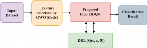
This section provides a simplified example of the ICL-DDQN framework's operational module. Figure 1 is a diagrammatic depiction of the suggested model.
Figure 1. Block diagram of the proposed methodology
3.1 Feature selection using grey wolf optimization (GWO)
The GWO is a new swarm intelligence algorithm that resembles the social structure and hunting strategy of gray wolves in the wild, as suggested by Mirjalili et al. [33]. Encircling, hunting, and assaulting prey are the main actions in this GWO. Wolves graded as alpha are the leaders which can be either male or female. They live as a family and they strictly follow social dominant hierarchy. GWO consist of four categories which are listed below.
Alpha (α): The male or female leader of wolves nominated as α are responsible for making decision over seeking place, hunting, etc.
Beta (β): Beta wolves being the strongest nominee for next α wolves, it plays the role of adviser and provides feedback to α.
Delta (δ): These wolves work as scouts and obeys the instructions of α and β. They are also responsible for warning the pack if any danger occurs.
Omega (ω): The lowest ranking wolf is ω, which has to obey all the dominant wolves.
The key benefits of the GWO method are that it does not need any particular input parameters and uses less memory than other metaheuristic algorithms of lower complexity. Many academics are motivated to apply GWO in various practical tasks such as relevant feature selection from big datasets, controller parameter tweaking, route planning, power dispatch issues, scheduling, and in other engineering domains. In this proposed system, GWO is used for the feature selection tasks from the collected datasets.
To illustrate, the matrix $N \times N$ matrix centered on the nth cell has the feature set $F=\left[f_{n-M} \ldots f_n \ldots f_{n+M}\right]$ and consisting of d-dimensional features fn in every column matching to $N=(2 M+1)$ cell for the selection task.
Encircling Prey
In this phase, the initial three wolves (represented by α, β and γ) in the optimal location (fittest solution) guide the other wolves represented by w toward promising regions of the search space. When hunting, grey wolves create a tight circle around their prey; during this time, each wolf's position (feature (Lf)) is updated using the aforementioned equations.
$\bar{L}=\left|\overrightarrow{M_f} \cdot \vec{X}_f(t)-\mu_f(\vec{X}(t))\right|$ (1)
$X_f(t+1)=\vec{X}_f(t)-\overrightarrow{A_f} \cdot \overrightarrow{L_f}$ (2)
Eq. (1) and Eq. (2) can be written as follows: let μf denote the mean calculation for feature, let $\vec{X}_f$ be the prey location (feature), let t denote the present iteration, and let $\vec{X}_f$ denote the grey wolf position (feature). In order to get the feature vectors $\vec{A}$ and $\vec{M}$ by using the formula:
$\overrightarrow{A_f}=2 \overrightarrow{k_f} \cdot \overrightarrow{r_1}-\overrightarrow{k_f}$ (3)
$\overrightarrow{M_f}=2 \cdot \vec{r}_2$ (4)
$\vec{r}_1, \vec{r}_2$ are random vectors between [0, 1] in equations Eq. (3) & Eq. (4), and components of ($\overrightarrow{k_f}$) linearly reduced from 2 to 0 throughout the number of repetitions.
Hunting
Mathematical models of grey wolf hunting behaviour take into account the roles of the α, β and γ packs, which only occasionally join in on the hunt themselves. If the candidate's best option is referred to by α, then β and γ will have more accurate knowledge of where their prey might be hiding.
After adjusting the positions of each wolf in the search space region using the geometric mean, the top three possible solutions are found. Following this, the best search agents' locations can be used to inform a random update of the locations of the remaining search agents around the prey (Eq. 5 through Eq. 9).
$\vec{L}_f(\alpha)=\left|\vec{M}_f(1) \cdot \vec{X}_f(\alpha)-\mu_f\left(\overrightarrow{X_f}(t)\right)\right|$ (5)
$\vec{L}_f(\beta)=\left|\vec{M}_f(2) \cdot \vec{X}_f(\beta)-\mu_f\left(\overrightarrow{X_f}(t)\right)\right|$ (6)
$\vec{L}_f(\gamma)=\left|\vec{M}_f(3) \cdot \vec{X}_f(\gamma)-\mu_f\left(\overrightarrow{X_f}(t)\right)\right|$ (7)
$\begin{gathered}\vec{X}_f(1)=\vec{X}_f(\alpha)-\vec{A}_f(1) \cdot\left(\vec{L}_f(\alpha)\right) \\ \vec{X}_f(2)=\vec{X}_f(\beta)-\vec{A}_f(2) \cdot\left(\vec{L}_f(\beta)\right) \\ \vec{X}_f(3)=\vec{X}_f(\gamma)-\vec{A}_f(3) \cdot\left(\vec{L}_f(\gamma)\right)\end{gathered}$ (8)
$\vec{X}_f(t+1)=\frac{\vec{X}_f(1)+\vec{X}_f(2)+\vec{X}_f(3)}{3}$ (9)
Attaching the prey
Wolf attacks on prey are represented by $\overrightarrow{k_f}$ which is randomly chosen and whose values will be between [-kf, kf]. The value $\overrightarrow{k_f}$ is lowered linearly over a limited number of iterations (2 to 0) as shown in Eq. (10).
$\overrightarrow{A_f}=2-t \cdot \frac{2}{\max { itns }} \overrightarrow{k_f}$ (10)
The aggregate number of feature selection iterations is max itns and iteration number is t.
Algorithm: GWO
Input: Extracted spectral features/classifier parameters from ConvLSTM
Output: Most optimal features
3.2 ICL- DDQN framework
The ICL- DDQN is composed of three sections which is briefly illustrated in below sections follows:
3.2.1 Structure of Conv-LSTM
The selected features from GWO are fed into Conv-LSTM. It efficiently transforms low-level to high-level features, which is then used to learn the distributed feature data representations. The efficient feature data representations assists the model in having comparable inputs with similar features as well as reducing dimensionality concerns, making it simpler to find patterns and anomalies and offering a better understanding of the overall model’s behavior. The explanation of Conv-LSTM is depicted below.
Assume, the cell state ct is the most crucial component of a conventional LSTM and is responsible for storing data. The input value Xt is saved if the input gate it is activated, while the prior state ct-1 is forgotten if the forget gate Ft is triggered. In addition, the final hidden state Ht is determined by whether the current cell state ct is converted or not by the output cell ot. The simplest LSTM model operates like this. When it comes to the ConvLSTM layer, however, everything from the inputs (tensors X1, X2, X, ....., Xn) to the cell states (tensors C1, C2, C3, ....., Cn) to the hidden states (tensors H1, H2, H3, ....., Hn) to the gates (i.e., it, ct, ot).
First, the inputs and gates are modelled as vectors on a grid in space; only then can the ConvLSTM layer's underlying working principle be grasped. The ConvLSTM layer predicts the upcoming state of a cell by aggregating the inputs and the previous state of the cell's local entities. Figure 2 depicts the internal organization of a Conv-LSTM cell.
Figure 2. Structure of ConvLSTM cell
The following set of Eq. (11-15) can help clarify this.
$f_t=\sigma\left(W_{X f} * X_t+W_{H f} * H_{t-1}+W_{C f} * C_{t-1}+b_f\right)$ (11)
$i_t=\sigma\left(W_{X i} * X_t+W_{H i} * H_{t-1}+W_{C i} * C_{t-1}+b_i\right)$ (12)
$o_t=\sigma\left(W_{X o} * X_t+W_{H o} * H_{t-1}+W_{C o} * C_{t-1}+b_o\right)$ (13)
$C_t=F_t \times C_{t-1}+I_t \times \tanh \left(W_{X C} * X_t+W_{H C} * H_{t-1}+b_c\right)$ (14)
$H_t=o_t \times \tanh \left(C_t\right)$ (15)
Convolution is denoted by ‘*’ and the Hadamard product is denoted by ‘×’, WCf, WCi, WCo and WHC indicates the weight matrixes. bf, bi, bo and bc, Each update will include a full recalculation of all weight matrices and bias vectors.
3.2.2 Reinforcement learning (RL) and Q-learning
Among the many facets of ML is reinforcement learning. In RL, the goal is to do the right action at the right time to maximize reward. The agent and the external world are the mainstays of the RL system, with which the agent has extensive interactions. The goal of RL is to have agents make decisions that are good for the environment as a whole. The selected action affects not just the immediate reinforcement value but also the future state of the environment and the eventual reward value.
The collection of actions that the agent should perform in each state is provided by the policy p in Eq. (16), where A is the set of states at each instant and S is the set of all spatial states; at and st are corresponding elements with time t. The term "optimal policy" refers to the process of determining which policy, or combination of policies, p* will produce the best results for a given situation.
$\pi: a_t \in A\left(s_t\right), s_t \in \mathrm{S}$ (16)
The compensatory procedure R is a reward signal that is calculated when performing activities in the environment. Timely assessment of a status. The agent's task is reflected in the reward function. It can also form the foundation of the agent adjustment policy. The value assigned to the activity is communicated via the reward signal. Eq. (17) describes the discount reward typically used in practice, where g is a discount factor and 0≤γ≤1. One prize is indicated by the letter r.
$R_t=r_{t+1}+\gamma \cdot r_{t+2}+\gamma^2 \cdot r_{t+3}+\cdots \cdot \sum_{k=0}^{\infty} \gamma^k \cdot r_{t+k+1}$ (17)
The value function, also called the evaluation function, is a metric for gauging the health of a system over the course of a lengthy period of time by comparing it to a desired future state. Under a certain policy p, the state-behavior value function resembles the Eq. (18), M stands for the mean.
$Q^p(s, a)=M_p\left\{R_t \mid s_t=s, a_t=a\right\}$ (18)
The value function under the optimal strategy is expressed by the following Eq. (19):
$Q^*(s, a)={ }_p^{\max } Q^p(s, a)$ (19)
Optimized by Bellaman equation, the accessible equation is depicted in Eq. (20):
$Q^*(s, a)=M\left\{r_{t+1}+\gamma \cdot \max _{a^{\prime}} Q^*\left(s_{t+1}, a^{\prime} \mid s_t,=s, a_t=a\right\}\right.$ (20)
Q-learning is a time-disparity model that can be used in place of an environment model; it is an RL algorithm. The predicted update of its best action value is based on a wide range of possible actions rather than the real actions selected based on the actual policy. It all comes down to thinking of the environment as a discrete state. Values for all possible actions in each state k of the learning process are characterized by a discrete Markov process and a function Q(s, a) is constructed decide the process. The recursive equation version of this statement is given by Eq. (21):
$Q_{k+1}\left(s_t, a_t\right)+a .\left(r_{t+1}+\gamma \cdot ^\max _p Q_k\left(s_{t+1}, a_{t+1}\right)-Q_k\left(s_t, a_t\right)\right)$ (21)
3.2.3 Employing DRL model in GWO-ConvLSTM for parameter optimization
The combination of RL and DL model is termed as DRL model. In this proposed system, the DRL is applied to adjust the parameters of ConvLSTM. The optimization process of DRL is divided into two parts:
·In RL part of DRL, the reward values will guide the parameter selection making reward-based optimization algorithm. The early Q-leaning uses a table to keep track of the reward value over all possible position states, and then uses that value to inform the next state decision.
In DL part of DRL, it is considered as the depth-enhanced learning as the table is replaced by the NN. The input of the state yields the appropriate decision result. The further state of NN is determined by its weighting parameters.
This optimization results have significant influence on the entire learning process and execution times for precise prediction rate.
3.2.4 DQN and DDQN
Both DQN and Q-learning are value iteration-based techniques. If the state and action spaces are discrete and the dimension is not too high, however, traditional Q-learning can still employ a Q-table to store the Q value of each state-activity. Using Q-table storage when both the state and the action space are high-dimensional continuous is difficult since the state and the action space are likely to be quite sizable. By fitting a function to generate Q values instead of a Q-table, let ensure that states with similar inputs receive similar outputs, effectively transforming the Q-table update into a function fitting problem. By integrating DL with RL, DQN is created and extracting complicated features using DNN.
Instead of using a Q-table to store the Q value, DQN predicts the Q value with the neural network and trains it on the best course of action all at once. DQN employs a two-network model architecture, with one network model (Qtraining) used to obtain the value of Q for training purposes, and the second network model (Qtesting) used to obtain the value of Q for evaluation. Similar to how DQN's primary and secondary networks are identical, so are Qtraining and Qtesting. The loss function l of DQN is graphically represented by Eq. (22):
$l(\vartheta)=M\left\{\left(Q_{ {testing }}-Q_{ {training }}\left(s_t, a_t, \vartheta\right)\right)^2\right\}$ (22)
$Q_{ {testing }}=r_{t+1}+\gamma \cdot a_{t+1}^{\max } Q_{ {testing }}\left(s_{t+1}, a_{t+1}, \vartheta^{-}\right)$ (23)
In Eq. (23), ϑ- is the parameter in the testing network. Standard Q-learning and DQN both use the max operation, which selects and measures an action based on the same variables. Since, DQN tends to be excessively-optimistic in selecting a high estimate could lead to an over-estimations values in the training data.
In this model, DDQN is developed to overcome the issues of DQN. In order for DDQN to be as effective as possible in removing the impact of overestimation, a straightforward operation must be carried out to separate the work of selecting the best action from the task of estimating the optimal action. DDQN employs two similar NN models. The first model learns during the experience replay much like DQN does. The second model copies the last episode of the first model. Decoupling the estimation allows DDQN to learn which states are (or are not) advantageous without having to figure out the effects of each action at each step, making it superior than DQN which also tends to reduce the complexity in the classification model. Eq. (24) provides the corresponding illustration.
$Q_{ {testing }}=r_{t+1}+\gamma Q_{ {testing }}\left(s_{t+1}, \operatorname{maxa}_{t+1} Q\left(s_{t+1}, s_{t+1} ; \vartheta\right) ; \vartheta^{-}\right.$ (24)
The above Eq. (24) illustrates the framework based on the improvement of DDQN.
3.2.5 Enhanced agent model
The complete model of this paper is based on DDQN, optimized ConvLSTM and Fully Connected (FC) layer. Incorporating state information into cell units is a strength of the optimized ConvLSTM. Briefly depicted in figure is a double-network framework, inside which are housed the training network and the testing network. Both the current state and the expected state in one minute from now are input into the training network. In the end, the error value is calculated by feeding the values determined by various networks into the loss function. The training network's parameters are adjusted according to the slope of the error, while the testing network's parameters are brought into lockstep with the former. When a final state is chosen, the corresponding parameters are written to memory d for later network modulation. The Figure 3 represents the schematic representation of integrating optimized ConvLSTM with DDQN model.
Figure 3. Schematic architecture of ConvLSTM with DDQN
Algorithm: DDQN
1. Set t=1
2. Start with a soft update of Experience Memory d and initialization with τ.
Use a random weight as ϑ the starting point for the training data.
Test data should begin with the primary network weights set to ϑ'.
3: for each episode do:
4: Initialize state st
5: for each time slot do:
6: In each st, choose an action (t).
7: Obtain reward r(t) and observe next state s'(t)
8: Solve (23) and obtain optimal action by DDQN
9: Store experience (s(t), a(t), r(t), s'(t) into d
10: Calculate the Q-value in testing network
11: If DRL=DQN, set test value
12: If DRL=DDQN, set test value
13. Train training network to minimize loss function
14. Update the testing network after few iterations
15. t=t+1
16: end for
17: end for
3.3 Classification
In order to accurately predict the cancer and its types, this framework adopts for the loss function which is represented by the Eq. (25):
$\left.l=M\left\{r+\gamma \cdot Q_{ {testing }}\left(s^{\prime}, \underset{a}{\operatorname{argmax}}\left(Q_{ {training }}\left(s^{\prime}, a\right)\right)\right)-Q_{ {training }}\left(s^{\prime}, a\right)\right)^2\right\}$ (25)
Eq. (25), defines the loss function to test whether the constructed model enhances the final prediction performance for the cancer and its types. If a loss function can be minimized to provide an improved margin classifier, then it can be used to create a more generic classifier. Improved generalizability and performance on unseen data can be achieved by increasing a classifier's margin. The generated loss function employed in this framework is a margin-enhancing loss function since it rewards incorrect data near the classification line.
In order to efficiently predict cancer, the GEM data is used to train and employ ICL-DDQN, which then selects the features and parameters that are most relevant.
4.1 Dataset description
The effectiveness of the suggested model has been demonstrated using data from three distinct cancer datasets, including breast cancer, lung cancer, and leukaemia, as shown in Table 1 below.
Table 1. Dataset observation
|
Dataset |
Instances |
Features |
Classes |
Reference |
|
Breast Cancer |
151 |
54676 |
6 |
[34] |
|
Leukemia |
72 |
7129 |
3 |
[35] |
|
Lung cancer |
181 |
12533 |
2 |
[36] |
4.2 Performance evaluation
This section assesses the efficacy of the ICL-DDQN model based cancer prediction method by implementing it in MATLAB 2019b. In this experimentation, different cancer dataset is taken for evaluation which is depicted in section 4.1. Of these, 65% of the data are taken for training, and 35% of the data are taken for testing. The Table 2 depicted the confusion matrix for different cancer prediction models.
Additionally, a comparative analysis is conducted between proposed and earlier models implemented on the considered literature: 1D-CNN [26], DL-DCGN [28] DL-SAE [29] and DL- AAA [31] regarding the following metrics:
Accuracy: The proportion of correctly labelled cases relative to the total number of examples. It is calculated by dividing the sum of true positives (individuals whose disease prediction was accurate) by the sum of true negatives (individuals whose health prediction was accurate). The formula is as follows:
$Accuracy=\frac{ { True \,\,Positive }(T P)+ { False\,\, Negative }(F N)}{T P+ { True\,\, Negative }(T N)+ { False \,\,Positive }(F P)+F N}$ (26)
Those without cancer are correctly labelled as healthy in TP, those with cancer in FP are wrongly labelled as healthy, those with cancer in TN are correctly labelled as healthy, and those with cancer in FN are incorrectly labelled as healthy in FN.
Precision: It calculates the properly classified instances at TP and FP rates.
$Precision=\frac{T P}{T P+F P}$ (27)
Recall: It defines the fraction of instances that are properly classified at TP and FN rates.
$Recall=\frac{T P}{T P+F N}$ (28)
F1-score: It is computed by:
$F=\frac{2 \times { Precision } \times { Recall }}{ { Precision }+ { Recall }}$ (29)
Average Error: It is the average error value obtained by proposed and existing classifiers to classify the GEM data.
Table 2. Confusion matrix
|
Methods |
Breast Cancer |
Leukemia |
Lung cancer |
|||||||||
|
TP |
TN |
FP |
FN |
TP |
TN |
FP |
FN |
TP |
TN |
FP |
FN |
|
|
1D-CNN |
25 |
27 |
13 |
10 |
10 |
11 |
10 |
5 |
33 |
34 |
15 |
8 |
|
DL-DCGN |
28 |
29 |
10 |
8 |
11 |
12 |
9 |
4 |
35 |
36 |
13 |
6 |
|
DL-SAE |
30 |
31 |
8 |
6 |
12 |
13 |
7 |
3 |
37 |
38 |
8 |
7 |
|
DL-AAA |
32 |
33 |
6 |
4 |
14 |
15 |
4 |
3 |
39 |
40 |
6 |
5 |
|
ICL-DDQN |
34 |
35 |
3 |
3 |
16 |
17 |
2 |
1 |
41 |
42 |
3 |
4 |
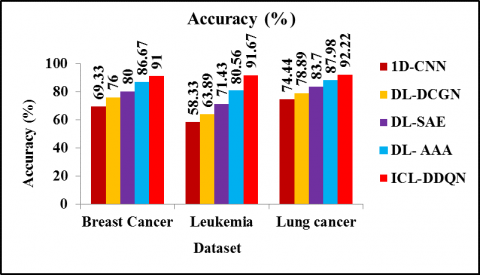
Figure 4 displays a comparison of the accuracy achieved by the ICL-DDQN, the 1D-CNN, the DL-DCGN, the DL-SAE, and the DL-AAA. According to the findings experiments, it is demonstrated that the proposed ICL-DDQN method has produced more accurate results than previously used methods for classifying microarray data. The accuracy of ICL-DDQN is 32.69%, 21.06%, 15% and 6.15% higher than 1D-CNN, DL-DCGN, DL-SAE, and DL-AAA. Similarly, the accuracy of ICL-DDQN is 57.16%, 43.18%, 28.33% and 13.79% greater than 1D-CNN, DL-DCGN, DL-SAE and DL-AAA method respectively for leukaemia. The accuracy of ICL-DDQN is 23.89%, 16.89%, 10.18% and 4.83% greater than 1D-CNN, DL-DCGN, DL-SAE and DL- AAA method for lung cancer dataset respectively. This is due to integration of GWO with Conv-LSTM model as it effectively learns the features data representation to reduce uncertainty and other systematic errors.
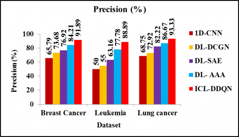
Figure 5 displays a comparison of the precision achieved by the ICL-DDQN, 1D-CNN, DL-DCGN, DL-SAE, and DL-AAA. Compared to 1D-CNN, DL-DCGN, DL-SAE, and DL-AAA, the precision of ICL-DDQN is 39.67%, 24.71 %, 19.46% and 9.12 % higher for breast cancer. Similarly, the precision of ICL-DDQN is 77.78%, 61.62%, 40.74% and 14.28%, greater than 1D-CNN, DL-DCGN, DL-SAE and DL-AAA method respectively for leukaemia. The precision of ICL-DDQN is 35.73%, 27.99%, 13.51% and 7.68% greater than 1D-CNN, DL-DCGN, DL-SAE and DL- AAA method for lung cancer dataset respectively. Therefore, it has been demonstrated that the suggested ICL-DDQN technique has higher precision rate as this model effectively train on the large sample instances for accurate results than previously used models.
Figure 4. Accuracy comparison for different cancer dataset
Figure 5. Precision evaluation for different cancer dataset
Figure 6 presents a recall-based performance evaluation of the ICL-DDQN, 1D-CNN, DL-DCGN, DL-SAE, and DL-AAA. The findings of the experiments show that when it comes to breast cancer, ICL-DDQN has a recall that is 28.64% higher than 1D-CNN, 18.14% higher than DL-DCGN, 10.27% higher than DL-SAE, and 3.37% higher than DL-AAA. Similarly, the recall of ICL-DDQN is 41.17%, 28.35%, 17.65% and 14.29% greater than 1D-CNN, DL-DCGN, DL-SAE and DL-AAA method respectively for leukaemia. The recall of ICL-DDQN is 13.43%, 6.95%, 8.57% and 3% greater than 1D-CNN, DL-DCGN, DL-SAE and DL- AAA method respectively for lung cancer dataset. When compared to other current models for classifying microarray data, the suggested ICL-DDQN technique was shown to produce superior results in terms of recall. As because, DRL finely optimizes the parameters of Conv-LSTM which intends the proposed model to make the optimal decisions for cancer classification.
Figure 7 displays a comparison of the F1-Scores obtained by the ICL-DDQN, the 1D-CNN, the DL-DCGN, the DL-SAE, and the DL-AAA. According to the data, ICL-DDQN outperforms 1D-CNN, DL-DCGN, DL-SAE, and DL-AAA in terms of F1-Score while analysing breast cancer, by 34.17, 21.41, 14.86, and 6.24 percentage points, respectively. Similarly, the F1-Score of ICL-DDQN is 60.02%, 45.45%, 29.52% and 13.95% greater than 1D-CNN, DL-DCGN, DL-SAE and DL-AAA method respectively for leukemia. The F1-Score of ICL-DDQN is 24.47%, 17.37%, 11.02% and 5.32% greater than 1D-CNN, DL-DCGN, DL-SAE and DL- AAA method respectively for lung cancer dataset. Therefore, it is demonstrated that the suggested ICL-DDQN technique for classifying microarray data outperforms previously-used models in terms of F1-Score. Since, DDQN model reduces the excessive estimations in the training data which smooth’s out the fluctuations, reduces the computational cost and boost the performance in the classification model.
Figure 6. Recall Comparison for various cancer dataset
Figure 7. F1-Score evaluation for different cancer dataset
The average error of 1D-CNN, DL-DCGN, DL-SAE, DL- AAA and ICL-DDQN is shown in Figure 8. Average errors for 1D-CNN, DL-DCGN, DL-SAE, and DL-AAA are 43.75%, 37.50%, 25%, and 10% lower than ICL-DDQN when 200 iterations are used. The results of this study show that the ICL-DDQN technique is superior to other proposed models for accurately predicting cancer. This is beacuse the DRL enhances decision-making and directly regulates the agents behavior through perceptual input learning.
Figure 8. Average error analysis for proposed and existing methods
In this study, an ICL-DDQN model is developed to choose the appropriate features using the GEM and optimizing the parameter simultaneously for accurate cancer prediction. The features are selected by using the GWO Model and employed the ConvLSTM to identify distributed feature representations in data by considering the high-level features. This model utilizes DRL to optimize hyperparameter of ConvLSTM and DDQN to eliminate overestimations in training data which significantly reduces the complexities and enhances the cancer detection performance. Experimental results show the proposed model outperforms state-of-the-art algorithms with 92.2%, 91.67%, and 92.22% accuracy for GEM based breast, leukaemia, and lung cancer datasets.
Thus, this model can be helpful for doctors and physicians to save their time and provides less focused manual inspections on large medical data, while also improving the decision-making process for earlier and more successful cancer treatments. On the other hand, the generalizability of this model was lower as it another important aspect which needs to be adjusted to increase the accuracy while minimizing the classification error. In future, a deep generative model will be developed for finding best genes and extract relevant gene expression features. Also, develop a novel methods based on specific attention mechanism for improving the structure of ICL-DDQN for the adaptability of analyzing various cancer datasets.
[1] Nath, A.S., Pal, A., Mukhopadhyay, S., Mondal, K.C. (2020). A survey on cancer prediction and detection with data analysis. Innovations in Systems and Software Engineering, 16(3): 231-243. https://doi.org/10.1007/s11334-019-00350-6
[2] Wang, H.Q., Jing, G.J., Zheng, C. (2014). Biology-constrained gene expression discretization for cancer classification. Neurocomputing, 145: 30-36. https://doi.org/10.1016/j.neucom.2014.04.064
[3] Ochs, M.F., Godwin, A.K. (2003). Microarrays in cancer: research and applications. BioTechniques, 34(S3): S4-S15.
[4] Liu, L., So, A.Y.L., Fan, J.B. (2015). Analysis of cancer genomes through microarrays and next-generation sequencing. Translational Cancer Research, 4(3): 212-218. http://dx.doi.org/10.3978/j.issn.2218-676X.2015.05.04
[5] Peng, Y., Wu, Z., Jiang, J. (2010). A novel feature selection approach for biomedical data classification. Journal of Biomedical Informatics, 43(1): 15-23. https://doi.org/10.1016/j.jbi.2009.07.008
[6] Elsebakhi, E., Asparouhov, O., Al-Ali, R. (2015). Novel incremental ranking framework for biomedical data analytics and dimensionality reduction: Big data challenges and opportunities. Journal of Computer Science & Systems Biology, 8(4): 203. http://dx.doi.org/10.4172/jcsb.1000190
[7] Kumar, M., Rath, N.K., Swain, A., Rath, S.K. (2015). Feature selection and classification of microarray data using MapReduce based ANOVA and K-nearest neighbor. Procedia Computer Science, 54: 301-310. https://doi.org/10.1016/j.procs.2015.06.035
[8] Bolón-Canedo, V., Sánchez-Marono, N., Alonso-Betanzos, A., Benítez, J.M., Herrera, F. (2014). A review of microarray datasets and applied feature selection methods. Information Sciences, 282: 111-135. https://doi.org/10.1016/j.ins.2014.05.042
[9] Yang, F., Mao, K.Z. (2013). Improving robustness of gene ranking by multi-criterion combination with novel gene importance transformation. International Journal of Data Mining and Bioinformatics, 7(1): 22-37. https://doi.org/10.1504/IJDMB.2013.050978
[10] Yang, F., Mao, K.Z. (2011). Robust FS for microarray data based on multicriterion fusion. IEEE/ACM Transactions on Computational Biology and Bioinformatics, 8(4): 1080-1092. https://doi.org/10.1109/tcbb.2010.103
[11] Kourou, K., Exarchos, T.P., Exarchos, K.P., Karamouzis, M.V., Fotiadis, D.I. (2015). Machine learning applications in cancer prognosis and prediction. Computational and Structural Biotechnology Journal, 13: 8-17. https://doi.org/10.1016/j.csbj.2014.11.005
[12] Osama, S., Shaban, H., Ali, A.A. (2022). Gene reduction and machine learning algorithms for cancer classification based on microarray gene expression data: A comprehensive review. Expert Systems with Applications, 118946. https://doi.org/10.1016/j.eswa.2022.118946
[13] Sumalatha, G., Kavitha, N.K. (2020). Enriched quantum artificial ant colony based breast cancer prediction. International Journal of Control and Automation, 13(1): 262–271.
[14] Sumalatha, G., Kavitha, N.K. (2022). Grey wolf enabled intuitionistic fuzzy CLARANS clustering for breast cancer prediction. Neuroquantology, 20(8): 4686-4694. https://doi.org/10.14704/nq.2022.20.8.NQ44496
[15] Gupta, S., Gupta, M.K., Shabaz, M., Sharma, A. (2022). Deep learning techniques for cancer classification using microarray gene expression data. Frontiers in Physiology, 2002: 952709. https://doi.org/10.3389/fphys.2022.952709
[16] Hanczar, B., Bourgeais, V., Zehraoui, F. (2022). Assessment of deep learning and transfer learning for cancer prediction based on gene expression data. BMC Bioinformatics, 23(1): 1-23. https://doi.org/10.1186/s12859-022-04807-7
[17] Ayyad, S.M., Saleh, A.I., Labib, L.M. (2019). Gene expression cancer classification using modified k-nearest neighbors technique. Biosystems, 176: 41-51. https://doi.org/10.1016/j.biosystems.2018.12.009
[18] Sharma, A., Rani, R. (2019). C-HMOSHSSA: Gene selection for cancer classification using multi-objective meta-heuristic and machine learning methods. Computer Methods and Programs in Biomedicine, 178: 219-235. https://doi.org/10.1016/j.cmpb.2019.06.029
[19] Xu, J., Wu, P., Chen, Y., Meng, Q., Dawood, H., Khan, M.M. (2019). A novel deep flexible neural forest model for classification of cancer subtypes based on gene expression data. IEEE Access, 7: 22086-22095. https://doi.org/10.1109/ACCESS.2019.2898723
[20] Wang, H., Tan, L., Niu, B. (2019). Feature selection for classification of microarray gene expression cancers using bacterial colony optimization with multi-dimensional population. Swarm and Evolutionary Computation, 48: 172-181. https://doi.org/10.1016/j.swevo.2019.04.004
[21] Shukla, A.K., Singh, P., Vardhan, M. (2020). Gene selection for cancer types classification using novel hybrid metaheuristics approach. Swarm and Evolutionary Computation, 54: 1-16. https://doi.org/10.1016/j.swevo.2020.100661
[22] García-Díaz, P., Sánchez-Berriel, I., Martínez-Rojas, J.A., Diez-Pascual, A.M. (2020). Unsupervised feature selection algorithm for multiclass cancer classification of gene expression RNA-Seq data. Genomics, 112(2): 1916-1925. https://doi.org/10.1016/j.ygeno.2019.11.004
[23] Shukla, A.K. (2020). Identification of cancerous gene groups from microarray data by employing adaptive genetic and support vector machine technique. Computational Intelligence, 36(1): 102-131. https://doi.org/10.1111/coin.12245
[24] Fathi, H., AlSalman, H., Gumaei, A., Manhrawy, I.I., Hussien, A.G., El-Kafrawy, P. (2021). An efficient cancer classification model using microarray and high-dimensional data. Computational Intelligence and Neuroscience, 2021: 7231126. https://doi.org/10.1155/2021/7231126.
[25] Lopez-Garcia, G., Jerez, J.M., Franco, L., Veredas, F.J. (2020). Transfer learning with convolutional neural networks for cancer survival prediction using gene-expression data. PloS one, 15(3): e0230536. https://doi.org/10.1371/journal.pone.0230536
[26] Mohammed, M., Mwambi, H., Mboya, I.B., Elbashir, M.K.,Omolo, B. (2021). A stacking ensemble DL approach to cancer type classification based on TCGA data. Scientific Reports, 11(1): 1-22. https://doi.org/10.1038/s41598-021-95128-x
[27] Zhong, L., Meng, Q., Chen, Y. (2021). A cascade flexible neural forest model for cancer subtypes classification on gene expression data. Computational Intelligence and Neuroscience, 2021: 6480456. https://doi.org/10.1155/2021/6480456
[28] Shen, J., Shi, J., Luo, J., Zhai, H., Liu, X., Wu, Z., Yan, C., Luo, H. (2022). Deep learning approach for cancer subtype classification using high-dimensional gene expression data. BMC Bioinformatics, 23(1): 1-17. https://doi.org/10.1186/s12859-022-04980-9
[29] Rezaee, K., Jeon, G., Khosravi, M.R., Attar, H.H., Sabzevari, A. (2022). Deep learning based microarray cancer classification and ensemble gene selection approach. IET Systems Biology, 16(3-4): 120-131. https://doi.org/10.1049/syb2.12044
[30] Rukhsar, L., Bangyal, W.H., Ali Khan, M.S., Ag Ibrahim, A.A., Nisar, K., Rawat, D.B. (2022). Analyzing RNA-seq gene expression data using deep learning approaches for cancer classification. Applied Sciences, 12(4): 1850. https://doi.org/10.3390/app12041850
[31] Kanwal, S., Khan, F., Alamri, S. (2022). A multimodal deep learning infused with artificial algae algorithm–An architecture of advanced E-health system for cancer prognosis prediction. Journal of King Saud University- Computer and Information Sciences, 34(6): 2707-2719. https://doi.org/10.1016/j.jksuci.2022.03.011
[32] Gangurde, R., Jagota, V., Khan, M.S., Sakthi, V.S., Boppana, U.M., Osei, B., Kishore, K.H. (2023). Developing an efficient cancer detection and prediction tool using convolution neural network integrated with neural pattern recognition. BioMed Research International, 2023: 6970256. https://doi.org/10.1155/2023/6970256
[33] Mirjalili, S., Mirjalili, S.M., Lewis, A. (2014). Grey wolf optimizer. Advances in Engineering Software, 69: 46-61. https://doi.org/10.1016/j.advengsoft.2013.12.007
[34] https://www.kaggle.com/datasets/brunogrisci/breast-cancer-gene-expression-cumida.
[35] https://web.stanford.edu/~hastie/CASI_files/DATA/leukemia.html.
[36] http://csse.szu.edu.cn/staff/zhuzx/Datasets.htm.