Manasa Chitradurga Manjunath*![]() | Blessed Prince Palayyan
| Blessed Prince Palayyan![]()
© 2023 IIETA. This article is published by IIETA and is licensed under the CC BY 4.0 license (http://creativecommons.org/licenses/by/4.0/).
OPEN ACCESS
Given India's vast expanse and dense population, the prediction of agricultural yields is crucial for ensuring food security. The task, however, is complex due to the influence of a multitude of factors, such as agricultural practices, environmental conditions, and technological advancements. Existing machine learning (ML) models face difficulties due to the quality and variability of data, model overfitting, intricate model structures, insufficient feature engineering, and temporal dependencies. Therefore, a robust and efficient model that addresses these challenges is imperative. In this study, an investigation was conducted using five prevalent ML algorithms — Random Forest (RF), XGBoost, Decision Tree (DT), Support Vector Machine (SVM), and Linear Regression (LR) — on a crop prediction dataset sourced from Kaggle. Algorithms that exhibited the highest coefficient of determination (R²) were selected to construct a hybrid model for aggregate prediction. Results demonstrated that the proposed hybrid model, encompassing DT, XGBoost, and RF, surpassed individual classifiers in terms of R² score and outperformed the existing models, achieving an accuracy of 98.6%. This provides a robust and efficient framework for crop yield predictions. Consequently, a user-friendly tool, 'Crop Yield Predictor', was developed, rendering the model accessible and practical for on-ground applications in agriculture. This tool effectively translates complex data and algorithms into actionable insights, bridging the gap between advanced machine learning techniques and practical agricultural applications.
machine learning, crop yield prediction, hybrid model, decision tree, support vector machine, random forest, gradient boosting, linear regression
Agriculture accounts for 60.45% of land use in India. Its agrarian economy stands as a cornerstone of its societal fabric, with agriculture deeply intertwined in its history and present. The nation's reliance on the annual monsoon and farming practices shapes the trajectory of its economy and the well-being of its populace [1]. As one of the most populous countries globally, India's ability to ensure food security hinges upon the efficacy of its agricultural yields. In this context, the accurate prediction of crop yields assumes paramount importance. On the one hand where farmers want timely guidance to anticipate crop output and establish effective methods to boost agricultural produce thereby earning better return on investments, Governments on the other hand must be able to accurately predict agricultural production to achieve national food security and make knowledgeable decisions regarding imports thereby saving crucial forex. To meet the increased food demands of India's burgeoning population, modern technology practices in agriculture are required.
Previously, farmers relied on their own experiences and accurate historical data to anticipate crop yields and make important production decisions based on the prediction. However, in recent years, new breakthroughs such as crop model simulation, precision agriculture, and machine learning have surfaced to estimate yield more precisely, as can analyze massive amounts of data using high-performance computing [2-5]. However, the task of predicting crop yields accurately is riddled with complexity. It entails the intricate interplay of a multitude of factors, encompassing agricultural methodologies, environmental variables, and technological advancements. The challenge is further compounded by the varied and often unpredictable nature of these variables, making traditional forecasting methods fall short in offering reliable predictions.
Precision agriculture [6], a revolutionary approach in modern farming, underscores the significance of targeted and data-driven cultivation practices. This methodology harnesses advanced technologies, including remote sensing, geographic information systems (GIS), and global positioning systems (GPS) as shown in Figure 1, to meticulously analyze and respond to the variability inherent in agricultural fields. By deploying sensors and data analytics, precision agriculture enables farmers to tailor irrigation, fertilization, and pesticide application precisely to the specific needs of different areas within a field. This approach not only maximizes crop yields but also minimizes resource wastage and environmental impact.
Figure 1. Components of precision agriculture
Statistical models, in comparison, provide a method that predicts direct connections between predictor variables and crop production within a particular dataset without taking into consideration underlying mechanisms in crop ecology and physiology [7]. When given adequate and trustworthy data, statistical models can make good predictions, but they may be constrained by the limits of the training data. However, widely used performance evaluation metrics are possible to get on statistical models that are helpful for uncertainty studies at regional scales and are less dependent on field calibration data. For forecasting agricultural yield, statistical models like multiple linear regressions (MLR) and simple linear regressions are frequently utilized [8].
There are a wide range of advantages to use machine learning (ML) models to forecast agricultural production. Machine learning places an emphasis on discovering patterns and correlations in data settings to precisely predict yields depending on various characteristics. ML models however must train on datasets that reflect previous experiences and results to create prediction models. Using historical data, the models' parameters are set during training. The performance of the model is evaluated during testing using a portion of the historical data that was not utilized for training [9]. Machine learning techniques have the capacity to adjust and learn from the nonlinear and dynamic processes of crop growth, which is essential for making precise forecasts for agricultural production. Due to learning ability from datasets, machine learning models are ideally suited for predicting agricultural yields at large scale. Further, their adaptability to different parameters like crop varieties, temperature, rainfall, humidity, nutrient content (nitrogen, phosphate, potassium, organic carbon, calcium, magnesium, Sulphur, manganese, and copper), pH levels and geographical area, make ML techniques them suitable to model and forecast crop yields [10].
While the potential of machine learning models to forecast crop yields holds promise, existing approaches have encountered a range of obstacles. Chief among these challenges is the dearth of comprehensive and high-quality data, the inherent variability within agricultural systems, the peril of overfitting intricate models, and the intricacies of temporal dependencies. Additionally, the models' efficacy has been hampered by the complexity of their structures and the insufficiency of thoughtful feature engineering.
Considering these hurdles, there emerges a compelling need for the development of more robust and efficient predictive models that can aid in the realm of sustainable crop production. Modern machine learning techniques such as hybrid or ensemble modeling, driven by their ability to make multiple models work together and handle complex and diverse datasets, present a transformative opportunity. Leveraging these tools could enable more accurate forecasts, assisting farmers, policymakers, and stakeholders alike in making informed decisions. In this paper, we harness the individual power of machine learning algorithms such as Decision Tree, XGBoost, Random Forest, Support Vector Machine, and Linear Regression using the agriculture dataset consisting of top 10 globally consumed crops from Kaggle repository. Choosing the top three algorithms in terms of performance, the study then exemplifies the fusion of these algorithms to propose a hybrid ML framework for efficient crop yield prediction and offer this as a tool for use of all stakeholders.
Therefore, the key contributions from this paper are:
The manuscript is organized as below: Section 1 provides an overview of crop yield prediction using machine learning and statistical models. Existing methods for agricultural yield prediction are reviewed in Section 2 under related works. Section 3 describes the materials and methods for agricultural yield prediction that have been offered. Section 4 contains the results and discussion. Section 5 concludes with references and draws conclusions.
In the field of crop yield prediction, numerous studies have been proposed mainly using machine learning algorithms compared to statistical or ensemble models. Authors [11] focus on predicting wheat yields using a combination of machine learning algorithms and advanced sensing technologies. The researchers explore how these methods can enhance the accuracy of predicting wheat yields, which is crucial for agricultural planning and management. The paper discusses the application of machine learning techniques along with advanced sensing tools to gather data relevant to wheat growth and yield. By analyzing this data, the study demonstrates how the combination of these technologies can lead to improved predictions of wheat yields, contributing to more informed decision-making in agricultural practices. Authors [12] explore the present and potential applications of statistical machine learning algorithms in agricultural machine vision systems. The authors discuss how these algorithms are currently being employed in various aspects of agriculture, specifically focusing on machine vision systems. They also highlight the potential future applications and advancements in this field, emphasizing the role of statistical machine learning techniques in improving agricultural processes and systems. The paper provides insights into the evolving landscape of agricultural technology and its integration with machine learning for enhanced efficiency and productivity. Authors [13] present a comprehensive survey on the integration of agrarian factors and machine learning models for yield forecasting. The authors delve into the various approaches that combine agricultural variables and machine learning techniques to predict crop yields. They examine the existing methodologies, discuss the challenges faced in yield forecasting, and assess the potential benefits of integrating agrarian factors with machine learning models. The paper offers insights into the state-of-the-art in yield prediction methods, emphasizing the importance of incorporating both domain knowledge and advanced machine learning techniques to enhance the accuracy of yield forecasts in agricultural contexts. The authors [8] discuss the application of Random Forests, a machine learning technique, for predicting crop yields at both global and regional scales. The authors explore the potential of Random Forests in improving crop yield predictions by integrating various data sources, including climate, soil, and remote sensing data. They demonstrate that Random Forests can effectively capture complex relationships between these factors and crop yields, leading to more accurate predictions. The paper highlights the importance of machine learning methods like Random Forests in enhancing our ability to forecast crop yields, which is crucial for global food security and agricultural planning. The authors [14] propose an ensemble method that combines multiple machine learning algorithms to create a more robust prediction model for crop production. They utilize various features and data related to crop growth and environmental conditions to train their model. By leveraging the strengths of multiple algorithms, the ensemble model aims to improve the accuracy of crop production predictions. The paper emphasizes the potential of ensemble techniques in enhancing the reliability of predictions in the agricultural context. Authors [15] focus on predicting crop yields through various machine learning algorithms. They discuss the methodology and results of employing these algorithms on datasets containing relevant agricultural information. The paper's objective is to showcase the potential of machine learning in forecasting crop yields, thereby contributing to improved agricultural planning and decision-making. Authors [16] focuses on predicting rice crop yields in India using support vector machines (SVM). They used relevant data related to rice cultivation, environmental factors, and historical yield records to train and validate their model. The paper aims to demonstrate the feasibility and accuracy of using SVM for predicting rice crop yields, which has implications for optimizing agricultural practices and food security in India. Authors [17] introduce an ensemble algorithm for predicting crop yields. The authors propose a method that combines multiple predictive models or algorithms to create a more accurate and reliable prediction for crop yields. They discuss the implementation of their ensemble algorithm, using various data sources related to crop growth, climate, and other relevant factors. The paper aims to showcase the effectiveness of ensemble techniques in improving the precision of crop yield predictions, contributing to better agricultural decision-making and planning. Authors [18] explore various supervised machine learning algorithms to develop predictive models for crop yield. They discuss how they utilized labeled datasets containing information about crop growth, environmental conditions, and other relevant factors to train and evaluate their models. The paper aims to demonstrate the applicability of supervised learning methods in accurately predicting crop yields, which can contribute to better agricultural planning and management strategies.
Authors [19] provide a comprehensive review of machine learning methods applied to crop yield prediction and nitrogen status estimation in precision agriculture. The authors likely survey various machine learning techniques used for predicting crop yields and estimating nitrogen levels in crops. They might discuss the strengths, limitations, and comparative effectiveness of these methods. The paper aims to summarize the state-of-the-art in using machine learning for precision agriculture tasks, emphasizing their potential in enhancing crop production efficiency and sustainability. As seen, there are very few studies leveraging hybrid ML models in literature.
In agriculture, crop yield prediction uses a variety of methods and tools to anticipate how much yield can be produced in a given area. The methodology includes obtaining information about the individual crop being farmed as well as environmental factors including weather patterns and resource availability. To anticipate agricultural yield, this data is subsequently examined using statistical models and machine learning techniques. The stages of data collection, pre-processing, feature extraction, model selection, training and prediction are commonly included in this work for crop yield prediction in agriculture.
Following exploratory analysis, four input variables (features in ML language) were identified: item, pesticide, rainfall, and temperature. The average crop yield was the variable to be anticipated. The mean and standard deviations of each variable in the training subset were used to standardize the data (i.e., subtract mean and divide by normal deviation). There are five unique features in the Kaggle dataset. Table 1 lists the feature descriptions for the dataset's various parameters. Figure 2 depicts the general design and workflow of the proposed system.
Figure 2. Overall architecture and workflow of the proposed framework
Table 1. Feature description in dataset
|
Feature |
Feature ID |
Description |
Dependent/ Independent |
|
Item |
Crop |
A total of 10 different crops were used in this dataset like paddy, wheat, maize etc. according to the country and the other factors that influence the crop growth |
Independent |
|
Pesticides (NPK) |
T (tonne) |
Data is collected from Food and Agricultural Organization (FAO) and active ingredients or pesticide usage is measured in tonnes |
|
|
Rainfall |
AAR (average annual rainfall) |
The average annual rainfall of different countries is measured in milli meters, and the data used was taken from world data bank |
|
|
Temperature |
AT (average temperature) |
Average temperature of particular year in particular region is measured in degree Celsius and world data bank helped in data collection |
|
|
Yield |
Y (tonne) |
The data is collected from FAO, and it is measured in tonnes |
Dependent |
3.1 Machine learning models
The ML models used in this work were chosen after doing a literature review. We use Random Forest, XGboost, Decision Tree, Support Vector Machines, and Linear Regression models, which are briefly described on how they are leveraged.
For a single independent variable (feature), mathematically, the linear regression equation is:
$y=b_0+b_1 * x+\varepsilon$ (1)
where:
- y is the predicted crop yield
- b0 is the intercept term
- b1 is the coefficient for the independent variable
- x is the value of the independent variable (e.g., weather
data)
- ε represents the error term
For multiple independent variables (features), the equation becomes:
$y=b_0+b_1 * x_1+b_2 * x_2+\ldots+b_n * x_n+\varepsilon$ (2)
where:
- x1, x2, ..., xn are the values of the independent variables (e.g., weather, soil properties, etc.)
- b1, b2, ..., bn are the corresponding coefficients for the independent variables
For crop yield prediction, we collect historical data that includes both input features (e.g., temperature, rainfall, soil nutrients) and the corresponding crop yield values. The goal of training the linear regression model is to find the coefficients (b0, b1, ..., bn) that minimize the difference between the predicted crop yields and the actual crop yields in the training dataset [20]. The training process involves using the least squares method to determine the optimal coefficients that best fit the data. Once the model is trained, we use it to predict the crop yield for new sets of input features by plugging them into the equation [21, 22].
The advantages of Linear regression are that it is a straightforward model that is easy to understand and implement. It provides a clear interpretation of the relationship between the independent variables and the dependent variable (crop yield). The coefficients in the linear regression equation provide insights into the direction and magnitude of the effect of each independent variable on the dependent variable. This can help in identifying which factors are most influential in predicting crop yield. These models are computationally efficient, making them suitable for quick analysis and prediction tasks, especially with a relatively small number of features. Linear regression doesn't assume a particular distribution of the data, which can be advantageous when working with different types of agricultural data. Linear regression at best serves as a baseline model, helping to establish a foundation for more complex modeling techniques if needed.
The drawbacks of Linear regression are that it assumes a linear relationship between independent and dependent variables. If the true relationship is non-linear, linear regression might not capture the complexity of the data accurately. Linear regression may struggle to capture intricate interactions and non-linear patterns present in crop yield data. Other models, like polynomial regression or machine learning techniques, might be better suited for such situations. Linear regression is sensitive to outliers, which can disproportionately influence the model's coefficients and predictions. Outliers are not uncommon in agricultural data due to various factors. When independent variables are correlated with each other, it can lead to multicollinearity issues in linear regression. This can affect the interpretation of coefficients and the model's stability. Without proper regularization techniques, linear regression can easily overfit (capture noise) or underfit (oversimplify) the data, leading to poor predictive performance. Linear regression assumes that the relationship between each independent variable and the dependent variable is independent of other variables. It might not handle complex interactions between features well. In cases where the relationship between variables is highly complex, linear regression might not provide accurate predictions. More advanced techniques may be required.
$H(S)=-\Sigma\left(P(c) * \log _2(P(c))\right)$ (3)
where, H(S) is the entropy of the dataset S, Σ denotes the sum over all possible classes c and P(c) is the proportion of instances in class c within the dataset S.
$I G(S, A)=H(S)-\Sigma\left(\left(\left|S \_v\right| /|S|\right) * H\left(S \_v\right)\right)$ (4)
where, IG(S, A) is the information gain of the dataset S by splitting on feature A, H(S) is the entropy of the original dataset S, Σ denotes the sum over all possible values v of feature A, |S_v| is the number of instances in the dataset S with feature A equal to v, |S| is the total number of instances in the dataset S and H(S_v) is the entropy of the subset S_v.
$I(S)=1-\Sigma\left(P(c)^2\right)$ (5)
where, I(S) is the Gini impurity of the dataset S, Σ denotes the sum over all possible classes c, P(c) is the proportion of instances in class c within the dataset S.
Figure 3. Representation of a decision tree implementation
The advantages of DT are that it provides a visual and intuitive representation of the decision-making process. The tree structure allows us to easily understand the factors and thresholds that contribute to predictions. They can capture non-linear relationships and interactions between variables in the data, making them suitable for complex agricultural systems where linear models might fall short. It can handle both categorical and numerical variables without the need for extensive preprocessing, which can be useful when dealing with diverse agricultural data. DTs are relatively robust to irrelevant features. Features that don't contribute significantly to prediction will tend to be pruned off during the tree-building process. They can handle missing values effectively by placing them in a separate branch during the tree-building process. DTs can be combined into ensemble techniques like Random Forests or Gradient Boosting, which often lead to improved predictive performance by reducing overfitting.
The drawbacks of DT are that they can become overly complex and fit noise in the training data, leading to poor generalization on new, unseen data. Small changes in the data can result in significantly different tree structures, making decision trees sensitive to variations and potentially leading to inconsistent predictions. In datasets with imbalanced classes, decision trees might have a bias towards predicting the majority class, especially if not adjusted appropriately. DTs use a greedy approach for building the tree, which might not lead to the globally optimal solution in some cases. Single decision trees can have high variance, especially on small datasets, which might require ensemble methods to mitigate this issue. While DTs can handle non-linearity well, they might not be the best choice for problems where linear relationships dominate. Preventing DTs from growing too deep or becoming too complex is important to avoid overfitting and maintain interpretability.
Step 1. Collect a dataset that includes historical data of crop yields and corresponding input features (e.g., weather data, soil properties, etc.). Randomly sample the dataset multiple times with replacement (bootstrap samples). Each sample is used to train an individual decision tree.
Step 2. For each bootstrap sample, build a decision tree using a subset of the input features. At each split node, randomly select a subset of features to consider for splitting. Split the data based on the selected feature that maximizes a certain criterion (e.g., information gain or Gini impurity) at that node. Repeat this process recursively until the tree is fully grown or a stopping criterion is met (e.g., maximum depth, minimum samples per leaf).
Step 3. Once all decision trees are built, predictions are made by aggregating the predictions of individual trees. For regression tasks like crop yield prediction, this aggregation is usually done by calculating the average of the predictions from all decision trees.
The mathematical representation of the Random Forest model is the ensemble average of individual decision tree predictions:
RandomForest $(x)=(1 / N) * \sum($ DecisionTree_$i(x))$ (6)
where:
- RandomForest(x) is the predicted crop yield for input features x using the Random Forest model.
- N is the number of decision trees in the ensemble.
- DecisionTree_i(x) represents the prediction of the i-th decision tree.
The advantages of RF for are that it reduces overfitting by combining multiple decision trees, which collectively make more robust predictions on new, unseen data. It can capture complex non-linear relationships between input features and crop yields. The model can provide insights into feature importance, helping to identify which factors contribute most to crop yield predictions and it is less sensitive to outliers and data noise due to the ensemble nature of the model.
The drawbacks of RF is that it can be computationally expensive and requires tuning to optimize performance. Although RF can indicate feature importance, the ensemble structure can make the model less interpretable compared to a single decision tree. While less prone to overfitting than individual decision trees, Random Forests can still overfit if the number of trees is too large relative to the dataset size.
Step 1. We collect a dataset containing historical data of crop yields and corresponding input features (e.g., climate data, soil characteristics, etc.).
Step 2. Define the SVM regression problem. In SVM regression, the goal is to find a hyperplane that best fits the data while minimizing the margin violations (deviations from the predicted values). Choose a kernel function (linear, polynomial, radial basis function, etc.) that maps the input features into a higher-dimensional space, allowing for more complex relationships between variables. Solve the optimization problem to find the coefficients of the hyperplane (weights) and the bias term that minimize the error while maximizing the margin between the predicted values and the actual crop yields.
The mathematical representation of the SVM regression model can be given as:
$y=w * x+b$ (7)
where:
- y is the predicted crop yield.
- w represents the weights (coefficients) of the hyperplane.
- x is the vector of input features.
- b is the bias term.
Step 3. Once the SVM regression model is trained, we use it to predict crop yields for new sets of input features.
The SVM regression model's objective is to find a hyperplane that best represents the relationship between the input features and crop yields. The prediction is made based on the distance of a new data point to the hyperplane.
The advantage of SVM Regression is that it can capture non-linear relationships between input features and crop yields using various kernel functions. SVMs generally have good generalization properties and can handle overfitting effectively. SVMs focus on the support vectors, which are the data points that influence the margin of error, making the model less sensitive to irrelevant features.
The drawback SVM Regression is that the training can be computationally intensive, especially with large datasets or complex kernels. SVMs have hyperparameters that require tuning, such as the choice of kernel, regularization parameter, etc. SVMs can be less interpretable compared to simpler models like linear regression and they might face challenges in terms of efficiency and scalability when dealing with massive datasets.
Step 1. We collect a dataset that includes historical data of crop yields and the corresponding input features (such as climate data, soil characteristics, etc.).
Step 2. Define the problem as a regression task, where the goal is to predict crop yields (a numerical value) based on input features. Install the XGBoost library and prepare the dataset in the required format.
Step 3. XGBoost has various hyperparameters that control the model's behavior. These include learning rate, maximum depth of trees, number of boosting rounds, regularization terms, and more. We perform hyperparameter tuning to find the optimal combination of these parameters that results in the best predictive performance. Techniques like grid search or random search can be used for this purpose.
Step 4. Train the XGBoost regression model on the dataset. The model works by sequentially adding decision trees to the ensemble, where each new tree tries to correct the errors made by the previous trees.
Step 5. Once the model is trained, we use it to predict crop yields for new sets of input features.
XGBoost is known for its accuracy and robustness, making it suitable for complex prediction tasks like crop yield prediction. It provides insights into feature importance, helping identify which factors are most influential in determining crop yields. It can capture complex non-linear relationships between input features and crop yields. Through hyperparameter tuning and regularization techniques, it can mitigate overfitting.
On the other side, setting up and tuning a model will require more effort compared to simpler algorithms. While it can provide feature importance, the model's ensemble nature can make it less interpretable than linear models.”
3.2 Methodology
The methodology adopted for crop yield prediction involves collecting and loading the data into a .csv file, followed by data pre-processing to handle outliers and selecting relevant features. The performance of the model is evaluated using appropriate metrics, and the predicted crop yields are displayed as the final output. Figure 4 shows the flow chart of the methodology adopted which is briefly explained below.
Figure 4. Flow-chart of the implementation
Data Collection and Loading. This involves importing all the requisite libraries in Python and loading the dataset from kaggle.com. We combine two datasets taken from http://www.fao.org/home/en/ and https://data.worldbank.org/. Feature description in the dataset is shown in Table 1. The dataset contains information on top 10 crops that are grown in USA. There are features like rainfall, temperature and pesticides that are included to determine the yield of the crops. There are around 28K records in the dataset.
Data Pre-processing. The collected data undergoes pre-processing to ensure data quality and integrity. We carry our exploratory data analysis (EDA) on the dataset to identify and select featured based on their relevance to the prediction task. Furthermore, an outlier removal process is applied to detect and eliminate any anomalous data points that could negatively impact the model's performance.
Model Training and Testing. Here, the dataset is divided into a train set and a test set, as well as into independent and dependent variables, or X and Y. 80% is the training data and 20% is the test data set split. Next, all the five ML models are trained using the train dataset and then the algorithm performance is checked on the remaining test data on all metrics. Based on best of three model performance on coefficient of determination (R2) score, we implement a hybrid ML framework.
Prediction and Evaluation. Once the hybrid ML models have been chosen and trained, they are ready to make predictions on new, unseen data. The input data is passed through all the trained models, and it generates predictions for the corresponding crop yield. Evaluation metrics are used to assess the performance of all the models and compare their predictive accuracy.
Output Display. The final step of the system design involves displaying the outputs, which include the predicted crop yields generated by the hybrid ML model. These predictions can be presented visually, such as in a graphical format, or as a tabular output showcasing the predicted yields for each input instance. Finally, a user-friendly interface is developed using the Gradio library in Python to view the predicted crop yield as per the inputs given by any user.
3.3 Evaluation metrics
The proposed models are evaluated using the following metrics.
$R M S E=\sqrt{\overline{(f-o)^2}}$ (8)
where, f= forecasts (expected values or unknown results), and o=observed values (known results).
$M A E=\frac{\sum_{i=1}^n\left|y_i-x_i\right|}{n}=\frac{\sum_{i=1}^n\left|e_i\right|}{n}$ (9)
It is thus an arithmetic average of the absolute errors $\left|e_i\right|=\left|y_i-x_i\right|$, where $y_i$ is the prediction and $x_i$ the true value.
Both the MAE and RMSE can range from 0 to ∞. They are negatively oriented scores. Lower values are better.
If a vector of n predictions is generated from a sample of n data points on all variables, and Y is the vector of observed values of the variable being predicted, with Y being the predicted values (e.g., from a least-squares fit), then the predictor's within-sample MSE is calculated as
$M S E=\frac{1}{n} \sum_{i=1}^n\left(Y_i-\hat{Y}_i\right)^2$ (10)
Lower the value the better and 0 means the model is perfect.
The results are segregated into three comparative studies, namely exploratory data analysis, intra-model and inter-model comparisons as discussed below.
4.1 Exploratory data analysis
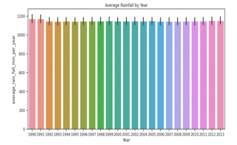
The results of EDA are first studied. Figure 5, Figure 6 and Figure 7 provide some valuable insights into the dataset like total pesticide usage by crops, average rainfall for by year and yield by item and year.
Figure 5. Total pesticide usage by crops
Figure 6. Average rainfall by year
Figure 7. Yield by item and year
4.2 Intra-model comparison
Results of all the models implemented in a standalone mode are shown in Table 2. It is observed that the R2 value of Random forest, Decision Tree and XGboost are highest in comparison to SVM and Linear regression indicating a perfect correlation. This is due to their ability to capture complex relationships, handle non-linearities, and address overfitting better compared to SVM and LR models. The SVM and LR models assume linear relationships between features and target variable yield. In the case of complex interactions or non-linearities, they struggle to capture the underlying patterns in the data, leading to lower R2 scores. Hence, DT+XGBoost+RF models are used for implementing the hybrid ML model.
4.2.1 Hybrid ML Model
The first model in the hybrid framework is the Decision tree regressor, second model is Gradient boosting regressor and third model is the Random forest respectively. We choose this order of models because of their roles and contribution to the overall model. Firstly, Decision trees make several important contributions to the hybrid ML model as they offer interpretability, facilitate feature selection, capture nonlinear relationships, enable ensemble learning, and handle missing data and outliers. These qualities enhance the accuracy, understanding, and applicability of the model for crop yield prediction. Secondly, Gradient Boosting Regression is a powerful algorithm which contributes by sequentially building models, handling non-linear relationships, providing feature importance analysis, robustness to outliers, regularization to control overfitting and offering some level of model interpretability. These contributions enhance the accuracy, reliability, and interpretability of the hybrid model. Random forest enhances the hybrid ML model by improving accuracy, robustness to noise and outliers, providing feature importance insights, handling high-dimensional data, enabling error estimation, and supporting parallel processing. These attributes contribute to more accurate and reliable predictions for crop yields, assisting in agricultural decision-making and resource management.
For training and testing the hybrid ML model, we use certain parameters like n-estimators and max depth. We optimize the results by hyper tuning these parameters. Table 3 indicates the parameter values which gave the best results.
Following the Decision Tree Regressor, the extracted features and the dataset are passed to the Gradient Boosting model. XGBoost is an implementation of Gradient Boosted decision trees. In this algorithm, decision trees are created in sequential form. Weights play an important role in XGBoost. Weights are assigned to all the independent variables which are then fed into the decision tree which predicts results. The weight of variables predicted wrong by the tree is increased and these variables are then fed to the second decision tree. These individual predictors then ensemble and for each candidate in the test set, it uses the class with the majority voting as the final prediction as shown in Figure 8. The output of the Gradient Boosting model is then fed into the Random Forest regression model as illustrated in Figure 9. Random Forest employs a decision tree as its base classifier. An attribute split/evaluation measure is used in decision tree induction to determine the best split at each node of the decision tree. The generalisation error of a forest of tree classifiers is determined by the strength of the individual trees in the forest as well as their correlation.
Figure 8. XGboost learning algorithm
First, a random forest is formed by selecting one of the five split measures at a time. For example, random forest with information gain, random forest with gain ratio, etc. Following that, a unique hybrid decision tree model for random forest classifier is developed. Individual decision trees in Random Forest are built in this model using various split measures. Weighted voting depending on the strength of individual trees augments this paradigm. This hybrid model's assessment metrics and correctness are scrutinized. Combining multiple decision trees enhances the accuracy and stability of predictions.
From results in Table 4, it is seen that the hybrid ML model returns the highest R2 value of 0.9847 compared to all individual models. Since various factors like temperature, rainfall, soil composition, and agricultural practices interact in complex ways, the hybrid model is better equipped to handle these intricate relationships and spatiotemporal nonlinearities present in the data and uses them effectively in predicting the yield. Also, the ensemble nature of RF by combining multiple DTs, feature importance measures, and XGBoost’s boosting mechanism contributes to higher R2 score of the hybrid model.
Figure 9. Hybrid decision tree model for random forest regression
Table 2. Intra-model experimental results
|
Metrics |
Random Forest |
Decision Tree |
SVM |
Linear Regression |
XGBoost |
|
R2 |
0.9837 |
0.9737 |
-0.2040 |
0.08628 |
0.9732 |
|
RMSE |
10645.42 |
13938.83 |
14083.62 |
94468.60 |
82295.73 |
|
MAE |
3999.17 |
4191.63 |
7954.61 |
57669.24 |
62779.32 |
|
MSE |
6772588013.10 |
194519546.09 |
198348525.23 |
8924316839.95 |
6772588013.10 |
Table 3. Hybrid ML model tuning parameters
|
Model |
N-Estimator |
Max Depth |
|
Decision Tree |
- |
10 |
|
Gradient Boost |
500 |
10 |
|
Random Forest |
500 |
11 |
Figure 10 illustrates the R2 scores comparison of all the algorithms, including the hybrid ML model. On comparison of all other metrics, the proposed hybrid ML model returns the lowest MAE, MSE and RMSE values by leveraging the complementary strengths of different algorithms, reducing bias and variance, capturing complex relationships, and creating an ensemble effect that improves predictive accuracy. MAE scores provide information about the difference between actual and predicted values. A lower MAE value indicates a more efficient model in predicting yield. The MSE score indicates the squared difference between true and predicted numbers. Computing the RMSE score helps measure the standard deviation of the residuals. The lower the MSE and RMSE scores, the better the model for calculating returns.
Table 4. Hybrid ML model results
|
Metrics |
Hybrid Model |
|
R2 |
0.9847 |
|
RMSE |
9037.8081 |
|
MAE |
3829.6532 |
|
MSE |
119182984.211 |
Figure 10. R2 scores comparison of all algorithms
4.3 Inter-model comparison
The proposed hybrid model is compared with existing models using various techniques on the same dataset. Table 5 shows the comparison in terms of model accuracy.
From inter model comparison results, the proposed hybrid model returns the highest accuracy of 98.6% thereby proving that the DT+XGBoost+RF model outperforms other state-of-the-art models compared with 4.47 pp better accuracy than the next best model. There are several potential improvements that could be made to the hybrid model to further enhance predictive accuracy. Feature engineering is one where quality and relevance of features can help improve model performance. By combining the right base models and different hyperparameter tuning can also help. Ensemble techniques like stacking can further optimize and improve accuracy. Applying regularization techniques to reduce overfitting in individual models by pruning decision trees or applying dropout in neural networks can help improve generalization and contribute to the hybrid model's accuracy.
Table 5. Inter model comparison results
|
Reference |
Model |
Accuracy (%) |
|
[23] |
Hybrid LSTM, RNN and SVM |
97 |
|
[24] |
Decision Tree |
84.54 |
|
[25] |
Deep Reinforcement Learning |
93.7 |
|
[26] |
Random Forest |
94.13 |
|
Proposed |
Hybrid DT for RF Regression using XGBoost |
98.6 |
Figure 11 and Figure 12 illustrate the Actual vs. Predicted yields for two crops, namely rice and wheat. The close alignment between the true & predicted values demonstrates the accuracy & reliability of the proposed hybrid model.
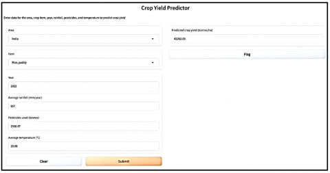
On account of superior model performance, an Industry use-case developed is a tool called ‘Crop Yield Predictor’ deployed with an easy user friendly interace that can be used by farmers, policymakers and other stakeholders for informed decision making as shown in Figure 13.
Figure 11. Actual vs. Predicted yield for rice
Figure 12. Actual vs. Predicted yield for wheat
Figure 13. The ‘Crop yield predictor’ user interface developed
A hybrid ML model is proposed for crop yiled prediction which combines the best three out of five ML models evaluated on their R2 scores, namely DT, XGBoost and RF. From results, the hybrid model outperforms the individual models implemented with an R2 score of 0.9847 and all others metrics like RMSE, MAE and MSE. In intra-model comparison with existing models, the proposed hybrid model outperforms them with an accuracy of 98.6%.
To ensure the accessibility of this model to policymakers and farmers at large, a user-friendly tool called ‘crop yield predictor’ is developed. Our findings contribute by offering a novel approach to predicting crop yield, advancing our understanding of hybrid modeling, providing insights into feature importance, and addressing practical challenges in agriculture and sustainability. The practical implications of the findings hold great potential for improving day-to-day agricultural operations and directly influence various aspects of agricultural decision-making for farmers and various stakeholders, enhancing productivity, sustainability, and economic outcomes for farmers. By translating complex data and algorithms into actionable insights, our findings bridge the gap between advanced machine learning techniques and practical on-ground applications in agriculture. As part of future research, we plan to investigate how temporal dynamics affect predictions. Also, we plan to incorporate crop disease, climate change and incorporate remote sensing data to capture spatial information about soil quality, vegetation health, and other factors that influence crop yield.
[1] Rashid, M., Bari, B.S., Yusup, Y., Kamaruddin, M.A., Khan, N. (2021). A comprehensive review of crop yield prediction using machine learning approaches with special emphasis on palm oil yield prediction. IEEE Access, 9: 63406-63439. https://doi.org/10.1109/ACCESS.2021.3075159
[2] Chlingaryan, A., Sukkarieh, S., Whelan, B. (2018). Machine learning approaches for crop yield prediction and nitrogen status estimation in precision agriculture: A review. Computers and Electronics in Agriculture, 151: 61-69. https://doi.org/10.1016/j.compag.2018.05.012
[3] Basso, B., Liu, L. (2019). Seasonal crop yield forecast: Methods applications and accuracies. Advances in Agronomy, 154: 201-255. https://doi.org/10.1016/bs.agron.2018.11.002
[4] Shahhosseini, M., Martinez-Feria, R.A., Hu, G., Archontoulis, S.V. (2019). Maize yield and nitrate loss prediction with machine learning algorithms. Environmental Research Letters, 14(12): 124026. https://doi.org/10.1088/1748-9326/ab5268
[5] Shahhosseini, M., Hu, G., Archontoulis, S.V. (2020). Forecasting corn yield with machine learning ensembles. Frontiers in Plant Science, 11: 1120. https://doi.org/10.3389/fpls.2020.01120
[6] Khosla, E., Dharavath, R., Priya, R. (2020). Crop yield prediction using aggregated rainfall-based modular artificial neural networks and support vector regression. Environmental Development and Sustainability, 22: 5687-5708. https://doi.org/10.1007/s10668-019-00445-x
[7] Van Klompenburg, T., Kassahun, A., Catal, C. (2020). Crop yield prediction using machine learning: A systematic literature review. Computers and Electronics in Agriculture, 177: 105709. https://doi.org/10.1016/j.compag.2020.105709
[8] Jeong, J.H., Resop, J.P., Mueller, N.D., Fleisher, D.H., Yun, K., Butler, E.E., Timlin, D.J., Shim, K.M., Gerber, J.S., Reddy, V.S., Kim, S.H. (2016). Random forests for global and regional crop yield predictions. PLoS ONE, 11(6): e0156571. https://doi.org/10.1371/journal.pone.0156571
[9] Walczak, S. (2016). Artificial neural networks and other AI applications for business management decision support. International Journal of Sociotechnology and Knowledge Development (IJSKD), 8(4): 1-20. https://doi.org/10.4018/IJSKD.2016100101
[10] Dahikar, S.S., Rode, S. (2014). Agricultural crop yield prediction using artificial neural network approach. International Journal of Innovative Research in Electrical, Electronics, Instrumentation and Control Engineering, 2(1): 683-686.
[11] Pantazi, X.E., Moshou, D., Alexandridis, T., Whetton, R. L., Mouazen, A.M. (2016). Wheat yield prediction using machine learning and advanced sensing techniques. Computers and Electronics in Agriculture, 121: 57-65. https://doi.org/10.1016/j.compag.2015.11.018
[12] Rehman, T.U., Mahmud, M. S., Chang, Y.K., Jin, J., Shin, J. (2019). Current and future applications of statistical machine learning algorithms for agricultural machine vision systems. Computers and Electronics in Agriculture, 156: 585-605. https://doi.org/10.1016/j.compag.2018.12.006
[13] Elavarasan, D., Vincent, D. R., Sharma, V., Zomaya, A. Y., Srinivasan, K. (2018). Forecasting yield by integrating agrarian factors and machine learning models: A survey. Computers and Electronics in Agriculture, 155: 257-282. https://doi.org/10.1016/j.compag.2018.10.024
[14] Balakrishnan, N., Muthukumarasamy, G. (2016). Crop production-ensemble machine learning model for prediction. International Journal of Computer Science and Software Engineering, 5(7): 148-153.
[15] Medar, R., Rajpurohit, V.S., Shweta, S. (2019). Crop yield prediction using machine learning techniques. In Proceedings of the 2019 IEEE 5th International Conference for Convergence in Technology (I2CT), Bombay, India, pp. 1-5. https://doi.org/10.1109/I2CT45611.2019.9033611
[16] Gandhi, N., Armstrong, L.J., Petkar, O., Tripathy, A.K. (2016). Rice crop yield prediction in India using support vector machines. In 2016 13th International Joint Conference on Computer Science and Software Engineering (JCSSE), Khon Kaen, Thailand, pp. 1-5. https://doi.org/10.1109/JCSSE.2016.7748856
[17] Keerthana, M., Meghana, K.J.M., Pravallika, S., Kavitha, M. (2021). An ensemble algorithm for crop yield prediction. In 2021 Third International Conference on Intelligent Communication Technologies and Virtual Mobile Networks (ICICV), Tirunelveli, India, pp. 963-970. https://doi.org/10.1109/ICICV50876.2021.9388479
[18] Suganya, M. (2020). Crop yield prediction using supervised learning techniques. International Journal of Computer Engineering and Technology, 11(2): 9-20.
[19] Chlingaryan, A., Sukkarieh, S., Whelan, B. (2018). Machine learning approaches for crop yield prediction and nitrogen status estimation in precision agriculture: A review. Computers and Electronics in Agriculture, 151: 61-69. https://doi.org/10.1016/j.compag.2018.05.012
[20] Freedman, D.A. (2009). Statistical Models: Theory and Practice. Cambridge University Press.
[21] Kavitha, S., Varuna, S., Ramya, R. (2016). A comparative analysis on linear regression and support vector regression. In Proceedings of IEEE International Conference on Green Engineering and Technologies (IC-GET), Coimbatore, pp. 1-5. https://doi.org/10.1109/GET.2016.7916627
[22] Huber, L.A., Xu, Q.B., Jürgens, G., Böck, G., Bühler, E., Gey, K.F., Schönitzer, D., Traill, K.N., Wick, G. (1991). Correlation of lymphocyte lipid composition membrane microviscosity and mitogen response in the aged. European Journal of Immunology, 21(11): 2761-2765. https://doi.org/10.1002/eji.1830211117
[23] Agarwal, S., Tarar, S. (2021). A hybrid approach for crop yield prediction using machine learning and deep learning algorithms. Journal of Physics: Conference Series, 1714(1): 012012. https://doi.org/10.1088/1742-6596/1714/1/012012
[24] Fayaz, S.A., Kaul, N., Kaul, S., Zaman, M., Baskhi, W.J. (2023). How machine learning is redefining agricultural sciences: An approach to predict apple crop production of Kashmir province. Revue d'Intelligence Artificielle, 37(2): 501-507.
[25] Elavarasan, D., Vincent, P.M.D. (2020). Crop yield prediction using deep reinforcement learning model for sustainable agrarian applications. IEEE Access, 8: 86886-86901. https://doi.org/10.1109/ACCESS.2020.2992480
[26] Pandith, V., Kour, H., Singh, S., Manhas, J., Sharma, V. (2020). Performance evaluation of machine learning techniques for mustard crop yield prediction from soil analysis. Journal of scientific research, 64(2): 394-398. https://doi.org/10.37398/JSR.2020.640254