Sunardi![]() | Anton Yudhana
| Anton Yudhana![]() | Miftahuddin Fahmi*
| Miftahuddin Fahmi*![]()
© 2023 IIETA. This article is published by IIETA and is licensed under the CC BY 4.0 license (http://creativecommons.org/licenses/by/4.0/).
OPEN ACCESS
Waste management, particularly waste sorting, constitutes a critical global challenge. The integration of advanced technology, specifically machine learning, offers potential solutions to this pressing issue. In this study, a convolutional neural network (CNN) model was employed to devise an efficient waste classification system. The model achieved notable results, attaining an accuracy rate of 98.92% and a loss percentage of only 4.03% in overall performance on the test set, utilizing the Kaggle dataset. To further improve the CNN model's performance, advanced preprocessing techniques were implemented alongside a stream lined CNN model, yielding substantial effectiveness. This investigation demonstrates that the application of machine learning techniques can result in highly accurate and efficient waste classification, presenting promising solutions for waste management challenges. By accurately identifying and sorting waste materials, this technology has the potential to significantly reduce the volume of waste directed to landfills, safeguard the environment, and conserve valuable resources.
waste classification, environmental management, recycling, CNN, deep learning
Waste poses significant impacts on daily human life and the environment [1]. Effective waste management is essential for addressing this issue, with waste sorting being a crucial component of the process [2]. Waste is typically categorized into inorganic, organic, and hazardous waste (B3) [3]. Upon sorting, each waste type undergoes appropriate processing: inorganic waste is recycled, organic waste is transformed into compost, and hazardous content within B3 waste is neutralized [3, 4]. Household waste, which primarily consists of organic and inorganic materials, is a common contributor to daily waste generation [5, 6].
The waste sorting process remains a challenge due to its time-consuming nature and the continuous growth of waste [7]. A prior interview conducted at a local waste bank revealed the need for a machine capable of sorting waste based on its type. One of the main hurdles faced by human sorters is the reluctance to endure prolonged exposure to the odor of waste. In contrast, machines can operate without concerns regarding the smell of garbage, making them ideal candidates for facilitating efficient waste sorting.
The development of a machine capable of classifying waste according to its type is essential for improving waste management efficiency. By employing machine learning techniques, such as convolutional neural networks (CNNs), designing an automated system that can accurately and efficiently differentiate between various waste types may be possible. This would streamline waste sorting processes and potentially mitigate the environmental impacts of waste accumulation.
Classifying waste images requires an appropriate classification method [8]. One of the classification methods that can be used is Convolutional Neural Network (CNN) [9]. CNN is a classification method in machine learning that uses many artificial neural networks and is commonly used for supervised machine learning [10]. CNN is commonly used to identify data in the form of images. The usual methods for CNN are convolution, pooling, dense, flatten, activation, and dropout [11]. These methods are often found in other classification methods, but what makes the CNN classification method unique are the convolution and pooling methods [12].
CNN implementation in machine learning requires a system that already has trained data based on the dataset [13]. The data was obtained from a dataset sourced from the Kaggle website [14]. Datasets from Kaggle can be preprocessed and simplified so that the machines can read the data [14].
The result of the implementation of CNN in machine learning is a machine that can classify images based on a predetermined type [15]. The reliability and effectiveness of the CNN classification method can be analyzed based on the accuracy and loss metric that occurs when classifying waste images [16].
Many previous studies have discussed machine learning for waste sorting using the CNN algorithm model. One of the studies is research conducted and published on the Kaggle website [17]. The research title is "Waste_classification CNN model," conducted by Bagchi [17]. The difference between Bagchi's and our research is the preprocessing and the CNN model used. The next difference is that Bagchi's research produces an accuracy of 87.10% and is still experiencing overfitting. In comparison, our study gets an accuracy of 98.92% without any overfitting seen in the analysis graph with data validation.
The following previous study is entitled Intelligent solid waste classification using deep convolutional neural networks, written by Altikat et al. [18]. This study describes the use and implementation of CNN to the problem of waste classification [18]. The difference between Altikat's and our research is the preprocessing and the complexity of the neural network. A comparison of the accuracy results in Altikat's research only reached 70% when using a five-layer neural network. The accuracy results obtained in our study was 98.92% which will be explained based on Table 1, Table 2 and Table 3.
Fahmi and Lubis [19] did a study on waste image processing in 2022, using the CNN algorithm to classify different forms of waste. The study had an accuracy rate ranging from 60% to 99%. With a 99% accuracy rate, bottles were the most accurately classified trash type utilizing CNN, followed by grass, which produced no real mistakes in the restricted system tested in this study. These findings point to the potential of CNN algorithm-based trash classification and management systems.
Shi et al. [20] investigated trash image processing in 2021, employing the CNN technique with Multilayer Hybrid feature extraction. According to the findings of this study, trash classification accuracy can reach up to 92.6%. These results indicate the efficacy of employing the CNN method in conjunction with Multilayer Hybrid feature extraction for waste classification using image processing.
Bobulski and Kubanek [21] published a study on waste image processing in 2019, leveraging the CNN algorithm to create a computer capable of capturing and detecting various sorts of rubbish. To achieve accurate trash classification through image processing, the researchers used both the AlexNet analytical model and their own analytical model. The results indicate the promise of CNN algorithm-based systems for garbage categorization and management, with 97% accuracy.
Based on many previous studies, the CNN model can be very effective for machine learning, especially for waste sorting cases. However, many only use RGB with various resizes in the preprocessing stage and still use complex CNN models.
The question from previous research is what makes the training data have the most accuracy and the most efficient classification model for handling datasets in the form of garbage images. The hypothesis believes that using complicated preparation procedures for training data can result in overfitting, primarily enhancing performance on the training data but potentially impeding generalization to new datasets. Furthermore, when image preprocessing exceeds the average level of complexity, it introduces extra distinguishing traits between objects that are beyond machine comprehension, hindering successful learning. In terms of classification models, the hypothesis posits that as the model's complexity increases, so does the time required for processing and training, potentially affecting classification performance.
The conclusion from the hypothesis is that each dataset has unique preprocessing and model complexity to achieve the desired efficiency level. Therefore, based on previous research, this study aims to determine the optimal image preprocessing techniques and CNN model complexity for effective waste classification.
This study employs a thorough methodology that includes data collecting, preprocessing procedures, and the creation of a Convolutional Neural Network (CNN) model. The dataset for this study came from Kaggle, a renowned online platform for data science competitions. It offers a wide range of images that can be used for training and evaluation. Gray-scale preprocessing techniques were used to improve data processing efficiency and reduce computational complexity. Color images are converted into grayscale representations using these techniques, which simplify the data while keeping crucial information. Finally, a CNN model was created that took advantage of its capacity to extract spatial hierarchies and patterns from images. The sections that follow go through each phase of the process in greater detail, emphasizing the importance of each component in attaining accurate and efficient classification results.
The majority of the methods employed in this study are quantitative in nature. The classification model's accuracy is a quantitative statistic, indicating that the data is numerical. The experts will examine the data and draw conclusions using mathematical and statistical tools. Although the primary focus of the research is a quantitative examination of classification model correctness, the researchers may also utilize qualitative approaches such as observation or interviews to gather information about the waste management process.
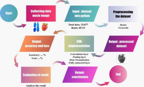
The research method was carried out sequentially, from data collection to evaluation. The following are the stages of the research method explained in Figure 1.
Figure 1. Research method flowchart
2.1 Dataset
The dataset is obtained by downloading from the Kaggle website [14]. The dataset consists of labeled data with two classes, usually called binary classes, namely inorganic and organic waste. The dataset contains training and test data with a total of 27,590 data. The total training data is 25,077 consisting of 13,966 organic waste images and 11.111 inorganic waste images. The total test data is 2,513 which consists of 1,401 organic waste images and 1,112 inorganic waste images [14]. The dataset was collected by Sekar in a JPG format file [14]. The training and validation data split size is 85:15 of the total data training. The training and test data split size is 85:15 of the total dataset. Preprocessing that is already done in the raw dataset is normalization, using a uniform format file which is JPG, and RGB color model.
2.2 Preprocessing
The following characteristics and procedures were used to efficiently process the enormous image dataset and solve the possible issues connected with its size. Grayscale Conversion: The decision to convert the photos to grayscale was motivated by a number of factors. For starters, grayscale images have only one channel of intensity information, which reduces computational complexity greatly when compared to color images, which have three channels (red, green, and blue). This simplification enables for faster CNN model processing and training. Second, grayscale photos can retain critical information for object detection and classification tasks, making them useful for a wide range of applications. Finally, gray-scale conversion reduces the influence of color changes and inconsistencies in the dataset, resulting in more robust and reliable feature extraction. Image Resizing: Resizing images to a certain dimension serves several functions. For starters, it aids in standardizing the input size for the CNN model. The algorithm can efficiently learn and recognize patterns and features throughout the dataset by scaling the photos to a consistent dimension. Second, by reducing the number of parameters and memory required for training the model, resizing minimizes the total computing overhead. This results in shorter training sessions and more efficiency. Furthermore, scaling can help offset the effects of the dataset's various image resolutions and aspect ratios, improving the model's capacity to generalize effectively to new and unknown images. This research used gray-scale conversion and image resizing techniques to optimize the preprocessing stage for the big image dataset, allowing for rapid and accurate training of the subsequent CNN model.
The preprocessing process is as follows. The dataset used is entered into an array using NumPy. The data is normalized using min-max normalization. Available labels are converted to numbers so the system can read them more efficiently [22]. The image is grayed out by adding a grayscale feature using cv2 [22]. The pixels are 50x50x1 because all images are resized to 50x50 pixels [22]. Variable 1 represents the image turned gray based on RGB to grayscale conversion formula explained in Eq. (1).
$Grayscale=(\text{R}+\text{G}+\text{B})/3$ (1)
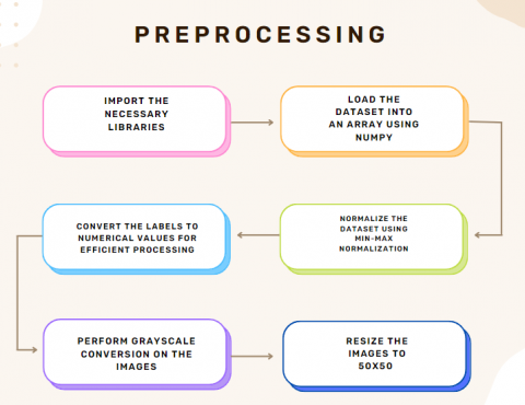
Figure 2. Preprocessing progress
Figure 3. Preprocessing flowchart
The size of all images in the dataset is changed to 50x50x1 pixels, and the image matrix is converted to one dimension array of 2500 8-bit pixels (flatten) [22]. The data is then shuffled to vary the categories [22]. Figure 2 shows the preprocessing of a dataset containing the waste image. Figure 3 shows the flowchart that summarizes the preprocessing stage.
2.3 CNN implementation
CNN consists of many neurons that are connected [23]. Each neuron has weight and bias values to predict image classification [24]. CNN is a deep neural network with two or more hidden layers [25]. The hidden layer of CNN consists of a convolution layer, a pooling layer, data normalization, and a fully-connected layer [26].
2.3.1 Convolution layer
The convolution layer is a layer that has a function to extract every feature in the image [27]. The convolution layer works by applying a 3x3 dimensional box to take and assess the weight and bias of each pixel in the image [28].
2.3.2 Pool layer
The pooling layer has a function to reduce the existing input parameters. It makes some of the data that is the core of the data taken. Another function is to reduce input resulting in faster data processing [29]. The pooling layer in our study uses max-pooling with a size of 2x2 with stride 2, which means that from every 2x2 pixel, the maximum value will be sought, and the maximum value will be output in an array forming a more superficial pool layer.
2.3.3 Data normalization
Data normalization is a layer that monitors the data involved in the machine-learning process [30]. The layer that is often used is flatten layer. Flatten layer is a layer that functions to change the dimensions of image data into one dimension uniformly [31].
2.3.4 Fully-connected layer
The fully-connected layer can connect the input layer, hidden layer, and output layer and activate the networks in the neural network [32]. Table 1 describes the CNN schema that occurs in this research.
The layer consists of Conv2D Layer with the following parameters and values. Layer sizes: 64, the kernel of Conv2D: 3x3, input Shape: 50x50x1, activation: ReLU.
The Conv2D layer performs convolutional operations on the input images. The layer has 64 filters, which means it will extract 64 different features from the input images. The kernel size is 3x3, indicating that the filters will operate on a 3x3 window. The input shape is 50x50x1, representing the resized grayscale images. ReLU activation is applied to introduce non-linearity, enabling the model to learn complex patterns and features effectively.
The next layer is MaxPooling2D Layer with the kernel: 2x2. MaxPooling2D reduces the spatial dimensions of the feature maps obtained from the previous Conv2D layer. It extracts the maximum value within each 2x2 window, effectively downsampling the features. This helps to reduce the computational complexity and retain the most prominent features.
The next layer is the Conv2D layer which consists of layer sizes: 64, the kernel of Conv2D: 3x3, and activation: ReLU. This Conv2D layer operates similarly to the first one, extracting additional 64 features from the previously downsampled feature maps. The second Conv2D layer also uses the MaxPooling2D layer with the kernel: 2x2. Another MaxPooling2D layer is applied to further downsample the features obtained from the second Conv2D layer.
The next layer is Flatten layer. The Flatten layer reshapes the 2D feature maps into a 1D vector, preparing the data for the subsequent fully connected layers.
Table 1. CNN schema
|
Parameter |
Value |
|
Conv2D (layer sizes) Kernel of Conv2D Input Shape Activation MaxPooling2D (kernel) |
64 3x3 50x50x1 relu 2x2 |
|
Conv2D (layer sizes) Kernel of Conv2D Activation MaxPooling2D (kernel) |
64 3x3 relu 2x2 |
|
Flatten Dense (layer sizes) Activation |
1D (default) 64 Relu |
|
Dense (layer sizes) Activation |
1 sigmoid |
|
Loss Optimizer Epochs Validation_split test_size |
binary_crossentropy adam 30 0.15 0.15 |
The next layer is the Dense layer which consists of layer sizes: 64 and Activation: ReLU. The first Dense layer is fully connected with 64 neurons. It performs high-level feature extraction and introduces non-linearity through ReLU activation.
The second Dense layer consists of layer sizes: 1 and activation: Sigmoid. The final Dense layer is the output layer with a single neuron, representing the binary classification task. Sigmoid activation is used to squash the output between 0 and 1, representing the probability of the input belonging to one class.
Additional Parameters consist of loss function: Binary Crossentropy, optimizer: Adam, epochs: 30, validation split: 0.15 (15% of the data used for validation during training), and test size: 0.15 (15% of the data used for testing the trained model). The binary cross-entropy loss function, which measures the difference between anticipated and actual class labels, is appropriate for binary classification tasks. Adam optimizer is a powerful optimization technique for neural network training. The model will be trained for 30 epochs, iterating 30 times over the dataset. For monitoring the model's performance during training, a validation split of 0.15 will be employed. Finally, a test set of 0.15 will be utilized to assess the model's ability to generalize on previously encountered data.
These design decisions and parameters are intended to promote effective feature extraction and classification, allowing the model to learn and generalize patterns from input photos using a simple architecture.
The CNN machine learning system was created with Python and the following software tools. NumPy is used for array operations and data manipulation. Pandas is a data analysis and manipulation framework. Image processing and visualization utilizing OpenCV for image reading and processing. Matplotlib is used to show images and create graphs. %matplotlib inline is a Jupyter Notebook magic command that displays plots inline. TensorFlow is used to build and train deep learning models, and it is used for model building and evaluation. Keras was used to create and configure the CNN model, which was imported from tensorflow.keras. For the train-test split, Scikit-learn was utilized.
2.4 Evaluation
Evaluation is the final stage of research which contains an analysis of research results in the form of a graphic diagram [33]. The graph displays the percentage of accuracy of training and validation data so that an analysis of the performance of the CNN classification method based on the waste image is formed [34]. After confirming that no overfitting happens, evaluate data training with the data test. After the overall results appear, a comparison of the experimental variables with previous research is carried out.
This research gives a detailed evaluation of the waste classification system in this section, comparing it to earlier works. The metrics and strategies utilized to evaluate the performance of the convolutional neural network (CNN) model are presented in this study. The following metrics were used to assess the performance of the waste classification system.
The accuracy rate is the percentage of waste samples that are accurately classified. It is determined as the number of successfully identified samples divided by the total number of samples.
The loss % shows the CNN model's overall performance. It is determined as a percentage of the loss sustained throughout the classifying process.
In the study, no precise thresholds were compared. This study, however, used THRESH_BINARY with a threshold value of 127 and a maximum value of 255.
This study used increased preprocessing approaches to improve the performance of the CNN model. Image preprocessing processes such as scaling, normalization, and data augmentation are likely to be used in this and earlier studies. These strategies try to improve the input data's quality and diversity, allowing the CNN model to train more successfully.
Unlike prior studies that used complicated CNN architectures, this study used a simpler CNN model. A simplified model could imply fewer layers or parameters. This option may aid in avoiding overfitting and improving generalization performance.
Bagchi's Investigation [17]: Bagchi conducted a waste categorization study utilizing the CNN algorithm, although the pretreatment procedures and CNN model employed in this investigation differed. Bagchi's study had an accuracy rate of 87.10% but suffered from overfitting. In comparison, without any overfitting, this study attained an accuracy of 98.92%. Figure 4, Figure 5, and Figure 6 will provide more information and a comparison of the analysis graphs with data validation.
Research by Alikat et al. [18]: Alikat's study focused on waste classification using CNN but with different preprocessing approaches and a more complicated neural network. Their study found that a five-layer neural network had an accuracy rate of only 70%. This study, on the other hand, attained an accuracy of 98.92%. Table 1 and Table 2 will provide a full comparison of accuracy outcomes.
Fahmi and Lubis [19] used the CNN algorithm for waste categorization in their work on waste image processing and achieved accuracy rates ranging from 60% to 99%. Bottles and grass had the best accuracy (99% and no read mistakes, respectively). These findings highlight the utility of CNN-based garbage classification systems.
Table 2. CNN scheme of Altikat's research (five-layer DCNN)
|
Parameter |
Value |
|
Conv2D Kernel of Conv2D Input Shape Activation MaxPooling2D (kernel)
Conv2D Kernel of Conv2D Activation MaxPooling2D (kernel)
Conv2D Kernel of Conv2D Activation MaxPooling2D (kernel)
Conv2D Kernel of Conv2D Activation MaxPooling2D (kernel)
Conv2D Kernel of Conv2D
Flatten Dense Activation
Dense Activation Validation_split test_size |
3x3 224x224x3 relu 2x2
3x3 relu 2x2
3x3 relu 2x2
3x3 relu 2x2
3x3
1D (default)
relu
1 Softmax 0.30 0.30 |
Research by Shi et al. [20]: Shi et al. investigated trash image processing utilizing the CNN algorithm with Multilayer Hybrid feature extraction. They attained up to 92.6% trash categorization accuracy. This study demonstrates the efficacy of employing the CNN method in conjunction with Multilayer Hybrid feature extraction for waste classification using image processing.
Bobulski and Kubanek [21]: Bobulski and Kubanek used image processing to classify garbage using the CNN method, including the AlexNet analytical model and their own analytical model. While exact accuracy rates were not provided, the researchers' findings indicate the promise of CNN-based systems for trash classification and management.
Overall, this research beats prior efforts in terms of accuracy and overfitting avoidance, proving the efficiency of improved preprocessing approaches and a simpler CNN model for trash classification used in this research.
The model evaluation phase produced informative data and outcomes that provide a full picture of the trained CNN model's performance and effectiveness. The model displayed amazing accuracy and efficiency in classifying photos into two categories: organic waste (O) and inorganic rubbish (R) after intensive testing and validation. The evaluation procedure included examining key parameters including accuracy and loss, which allowed for a complete examination of the model's predictive capabilities. Furthermore, the model underwent extensive validation to confirm its resilience and generalizability to new and previously unexplored data. The results reported in this section shed light on the model's ability to extract crucial features from preprocessed photos and accurately classify waste objects, therefore contributing to waste management and environmental sustainability.
Model evaluation metrics include "accuracy" and "binary cross-entropy loss." In classification tasks, accuracy is a typical evaluation parameter. The proportion of correctly categorized samples in the test set is calculated.
Accuracy in waste categorization refers to the percentage of waste items accurately classified by the model. Higher accuracy ratings suggest that the model is more accurate and trustworthy.
Binary cross-entropy is a frequent loss function for binary classification issues. It measures the difference between the anticipated probability distribution and the actual binary labels. The smaller the loss value, the more accurate the predicted probabilities are. Reduced binary cross-entropy loss allows the model to learn to produce more accurate predictions.
These metrics provide useful information about the waste classification model's performance. Accuracy aids in evaluating overall classification performance, whereas binary cross-entropy loss measures the model's prediction accuracy. You can assess the model's performance and dependability in correctly categorizing trash items by monitoring these metrics during training and analyzing them on the test set.
It should be noted that these metrics are typically utilized in binary classification jobs with two unique classes (in this case, waste or non-waste). Different assessment metrics, such as categorical cross-entropy or F1 score, may be employed if the classification problem comprises numerous classes.
In image processing, the THRESH_BINARY approach is a typical thresholding method. It divides a picture into two categories based on a threshold value. Pixels with intensity values less than the threshold are assigned the lowest value (0), whereas pixels with intensity values greater than or equal to the threshold are assigned the maximum value (255 in this case). This binary separation is ideal for jobs that require a clear differentiation, such as garbage classification.
The value 127 was chosen on the idea that it efficiently differentiates trash and non-waste regions in grayscale images. This particular value could have been derived via experimentation or domain knowledge. Finding a suitable threshold that best distinguishes between the two classes is critical for correct categorization.
In the thresholded image, the maximum value of 255 is chosen as the upper limit for pixel intensities. This value denotes the highest level of intensity, which is often used to highlight or emphasize the areas of interest. Setting the non-waste regions to the greatest value in this example aids in visually distinguishing them from the garbage regions in the final thresholded photos.
The research seeks to successfully differentiate waste and non-waste regions in photos by employing the THRESH_BINARY approach with a threshold value of 127 and a maximum value of 255. This thresholding method simplifies the image representation and focuses on the fundamental features that identify trash objects, making the subsequent classification work easier. It is crucial to note, however, that the choice of thresholding techniques and values may vary depending on the unique dataset and desired classification output, and additional research and optimization may be required to determine the most appropriate thresholding parameters.
The following are the results of the CNN schema execution based on the parameters listed in Table 1 with epochs are 30, with a dataset consisting of 25,077 waste images with the ratio of data training and data validation being 85:15.
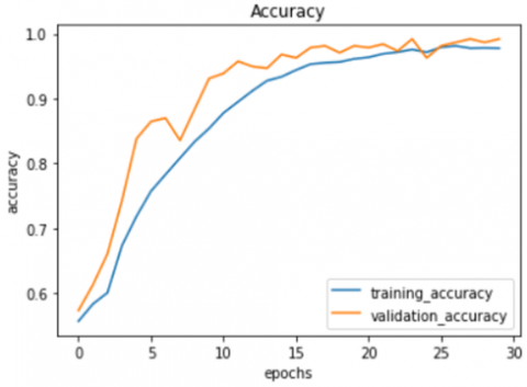
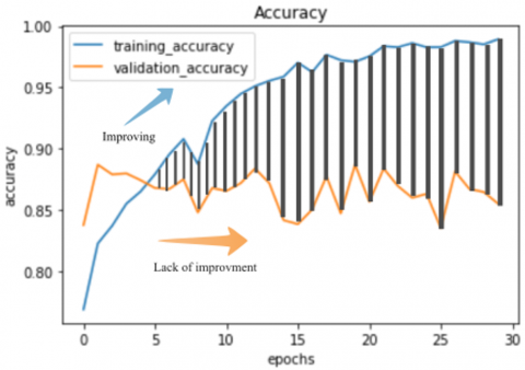
Figure 4 and Figure 5 show two graphs of training and validation data performance analysis. Figure 4 shows a graph of machine accuracy for data classification; accuracy between training and data validation is less than 5% in each epoch. It shows that the training data and data validation are average because every time the training data has been improved, the data validation has also improved. Suppose the difference between the training and validation data is too significant at some point based on the accuracy results because the validation data does not improve while the training data is still improving; the model is overfitting [35].
Figure 4. Accuracy result
Figure 5. Loss result
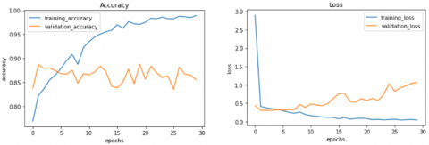
Overfitting is when performance is excellent on training data, but other data is still lacking [36]. Overfitting occurs because the accuracy of the training data needs to be more precise in classifying but cannot classify waste images in general [37]. It can be found in Bagchi's research [17].
Figure 6. Accuracy and lost result of Bagchi's research
Figure 7. Range of overfitting
Figure 7 shows that the average amount of training data accuracy reduced by the average number of validation data produces a performance difference where overfitting occurs at a particular percentage difference Eq. (2). Overfitting starts at epoch 5, and maximum overfitting happens at epoch 25. Overfitting only happens when validation data does not improve while the training data is still improving.
$\frac{\sum(X \mathrm{ti}-X \mathrm{di})}{(\mathrm{En}-\mathrm{Ea})}=\mathrm{O}$ (2)
where, $X_{\mathrm{ti}}$ is the accuracy of training data on the ith epoch, $X_{\mathrm{di}}$ is the accuracy of validation data on the ith epoch, En is the number of epochs that happen, and Ea is the first epoch where overfitting occurs. The result is O, where O is the percentage value of overfitting based on the average difference between the accuracy of training and validation data. Eq. (2) only applies if the validation data does not improve while the training data is still improving.
There are many analyses about overfitting, but none of the formulas explains overfitting. The only formula known now is when to stop the learning process before becoming overfitting based on the speed of the learning rate, called early stopping Eq. (3) and Eq. (4). The learning rate will become slower and stops when the value of training data keeps improving while other data does not improve.
$\frac{\partial C}{\partial Wj}=\frac{1}{n}\sum\limits_{X}{X}j(\sigma (z)-y)$ (3)
$\frac{\partial C}{\partial b}=\frac{1}{n}\sum\limits_{X}{(\sigma (z)-y)}$ (4)
$\frac{\partial C}{\partial W j}$ and $\frac{\partial C}{\partial b}$ are two partial derivatives of the cost function, determining the neuron's learning rate [36]. Wj is the value of the jth weight, C is the cost, b is the bias, Xj is the jth input, and y is the output [36]. From this formula, only at what point to stop the learning process is known, but we cannot determine what variable makes the dataset overfitting. Based on Figure 6, it starts overfitting at epoch five and will stop around epoch five if implementing the early-stopping formula in the syntax. The following figure shows the result of early stopping based on Figure 6 cases.
The percentage of a graph of overfitting cases has yet to be determined in the general formulation. Likewise, any variables that make the dataset experience overfitting. So far, many researchers still rely on analysis from graphs to find out, so the general determination of how large the percentage difference can be classified as overfitting still needs to be discovered. The percentage difference between training and validation data can be a constant that must be examined together with what constants are appropriate for average and overfitting data conditions. The second possibility is that variables can affect changes in the average difference between training and validation data, so this variable must be determined and formulated to form a formula for determining whether the data is average or experiencing overfitting.
Overfitting happens when a model grows overly complicated and begins to memorize the training data, resulting in poor generalization of previously unseen data. The following is a more in-depth overview of how overfitting was diagnosed, overfitting signs, and the implementation of early stopping.
Overfitting can be detected by tracking training and validation loss and accuracy during the model's training process. Overfitting is usually indicated by a considerable discrepancy in performance between the training and validation sets. If the training loss continues to fall while the validation loss begins to rise or plateau, this indicates that the model is overfitting and not generalizing well to new data.
When the training loss continues to drop while the validation loss remains reasonably high or begins to grow, this is an indication of overfitting. Another indicator is a considerable gap in training and validation accuracy, where the model achieves near-perfect accuracy on the training set but struggles on the validation set.
Early stopping was used as a regularization approach to combat overfitting. It prevents the model from over-optimizing the training data by terminating the training process when the model's performance on the validation set begins to worsen. This study established a validation loss or accuracy threshold at which training is halted to avoid overfitting.
Early stopping aids in determining the ideal point during training at which the model achieves good performance on both the training and validation sets, resulting in greater generalization to unknown data.
The authors intended to achieve a balance between model complexity and generalization by diagnosing overfitting, detecting its signs, and adopting early stopping. Early stopping prevents overfitting and enhances the model's capacity to perform effectively on unseen data. Figure 6. shows visualizations exhibiting overfitting that provides further evidence and insights into the model's behavior during training.
The theory that determines what variable affects the model to be overfitting or can improve the accuracy can be obtained from comparing the parameters between the previous study, which is Bagchi's study, and our study. Two main differences occur in the preprocessing parameters, namely the resize section and the color scale of the training data. In our study, the resize used was 50 pixels, while the previous study used 200 pixels. Then the color scale used in our study is grayscale, while the previous research is RGB. It shows that the input shape used is different; in our study, the input shape is 50x50x1, 1 indicates the color scale used is grayscale based on Eq. (1) while the previous research has 200x200x3, 3 indicates the color scale used is RGB based on Eq. (1).
Most previous journals claimed that resizing could affect the performance of the CNN model [38, 39]. It was also explained that the most effective resizing is a size close to the original image size [38]. So, there is no correlation. If the size is bigger, then the performance of the CNN model will be even more outstanding. There is also a theory that the larger the size value, the greater the accuracy and the more time used, especially when using the CNN model [39]. However, our study contradicts the two opinions because in our study, the average size of the original image is above 200x200 pixels, so it is not fulfilled for the first and second opinions because research has better accuracy using 50x50 pixels rather than 200x200 pixels. Resizing will have an effect, but the indicator that makes the performance better is the suitability of the size of the data image for a particular dataset, different datasets used will also have different efficient image sizes.
Figure 8. Example of the graph when implementing early stopping
Most previous journals also claimed that grayscale would work better [40]. However, many studies still use RGB [18, 41, 42]. The case study using the same dataset as the study [17] shows a difference in color scale. In research [17], they use RGB so that the final variable input shape entered into the CNN model is 3, while in our study, this research use grayscale so that the final variable input shape entered into the CNN model is 1. Grayscale has better performance and is also more efficient in its use [40]. The accuracy in classifying by the machine will increase if the object has a transparent edge and contrasts color with the background. The convolutional can give weight and bias value with a smaller range due to the limited color available while the contrast is still maintained. However, this opinion still needs improvement when comparing different datasets and models. The use of grayscale can be more effective if using specific datasets and RGB if done on other datasets [18, 40-45 ]. The following is Figure 8 explaining early-stopping when implemented into machine learning. It shows that early stopping only stops machine learning when overfitting might happen.
The following comparison is the CNN model based on the neural network's architecture.
Table 3. CNN scheme of Bagchi's research
|
Parameter |
Value |
|
Conv2D (layer size) Kernel of Conv2D Input Shape Activation MaxPooling2D (kernel)
Conv2D (layer size) Kernel of Conv2D Activation MaxPooling2D (kernel)
Conv2D Kernel of Conv2D Activation MaxPooling2D (kernel)
Flatten Dense (layer size) Activation
Dense (layer size) Activation Validation_split test_size |
32 3x3 200x200x3 relu 2x2
64 3x3 relu 2x2
128 3x3 relu 2x2
1D (default) 150 relu
1 Sigmoid 0.50 0.50 |
A comparison of the CNN model between the three studies (Table 1, Table 2, and Table 3.) can be seen from the number of layers built. The more layers used, the more complex the machine classifies objects. The level of model complexity can affect machine learning performance if the existing dataset is limited [46]. Several studies explain that the more complex a model is, the more vulnerable it will be to reduced accuracy performance [46]. However, some argue that complex models can improve machine learning performance because the function of complexity can solve problems that occur [47]. For example, CNN combined with LSTM will be good because the function of the two models, such as CNN as a model that functions as a recognition skill, LSTM as a model that provides time series data, and the combination serve as a calculation speed in problem-solving [44]. This study (Table 1), compared to the study (Table 2), had better accuracy results even though the depth and complexity of the neural network were more straightforward in this study. The complexity and depth of the CNN model architecture have an influence, but each dataset has a unique value, so it cannot be applied to different datasets.
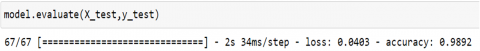
After the result of training data compare with validation data is no resulting overfitting, the next step is to see the accuracy result tested using test data. The acquired result is an accuracy of 98.92% and loss of 4,03%. Figure 9 is the result of evaluating machine learning using test data.
The three CNN models mentioned in Table 1, Table 2, and Table 3, prior research by Fahmi and Lubis [19], Shi et al. [20], and Bobulski and Kubanek [21], we can look at model architecture, hyperparameters, performance metrics, and overfitting. The three CNN models in the table differ in terms of model design, including the amount of Conv2D and Dense layers, their sizes, and the usage of additional layers such as MaxPooling2D and Flatten.
Fahmi and Lubis [19] design produced an accuracy rate ranging from 60% to 99%. Shi et al. [20] used the CNN technique with Multilayer Hybrid feature extraction, whereas Bobulski and Kubanek [21] used the AlexNet analytical model as well as their own.
Figure 9. Result with test data
Each CNN model in Table 1, Table 2, and Table 3 and earlier research had distinct hyperparameter values, including kernel sizes, input shapes, activation functions, and optimization strategies, based on hyperparameters.
According to Table 1, Table 2, and Table 3 performance metrics, the CNN models achieved binary cross-entropy loss and employed accuracy as a performance parameter. Fahmi and Lubis [19] observed trash classification accuracy rates ranging from 60% to 99% using their CNN algorithm. Shi et al. [20] used the CNN method with Multilayer Hybrid feature extraction to achieve waste categorization accuracy of up to 92.6%. Bobulski and Kubanek [21] specific performance measurements have up to 97% accuracy. This study assumes that only Bagchi's work is overfitting because it appears very clearly in Figure 6, while other work doesn’t show any evidence.
Differences in the results obtained from the models and studies can be attributed to various factors, including variations in model architectures, hyperparameter values, dataset characteristics, and data preprocessing techniques. Additionally, variations in the performance metrics used and the specific waste classification tasks tackled by each study could contribute to the differences observed.
However, when compared to the machine learning time required to classify, it is calculated that this research could be faster. One of the most significant factors that causes time to slow down is the ability of the computer to execute syntax commands. In this study, the computers used had specifications incapable of carrying out heavy executions, especially on the display device. Here are the specifications of the computer used. System Manufacturer: LENOVO, System Model: 10HV002JIA, BIOS: LENOVO BIOS Rev: M0KKT17A 0.0 (type: BIOS), Processor: Intel(R) Core(TM) i3-4170 CPU @ 3.70GHz (4 CPUs), ~3.7GHz, Memory: 4096MB RAM, Available OS Memory: 4006MB RAM, Page File: 3923MB used, 1553MB available, and the display device specification is ard name: Intel(R) HD Graphics 4400, Manufacturer: Intel Corporation, Chip type: Intel(R) HD Graphics Family, DAC type: Internal, Device Type: Full Device (POST), Device Problem Code: No Problem, Driver Problem Code: Unknown, Display Memory: 2115 MB, Dedicated Memory: 112 MB, Shared Memory: 2002 MB, Current Mode: 1440 x 900 (32bit) (60Hz), HDR Support: Not Supported, Display Topology: Internal, Display Color Space: DXGI_COLOR_SPACE_RGB_FULL_G22_NONE_P709, Color Primaries: Red(0.653320, 0.336914), Green(0.322266, 0.610352), Blue(0.151367, 0.064453), White Point(0.313477, 0.329102), Display Luminance: Min Luminance=0.5000000, Max Luminance=270.000000, MaxFullFrameLuminance=270.000 000.
The value is inversely proportional to accuracy compared with the loss percentage, like in Figure 5, because the validation data is greater than the training data. This incident proves that a good result of any classification method is when the accuracy percentage has a high value. In contrast, the loss percentage has a small value while training and validation data keep improving every epoch.
The test data results also show that our research's accuracy is better than previous studies using preprocessing and the previously described model with a value of 98.92%. It also shows that the garbage dataset [14] is more efficient using the same preprocessing parameters and CNN model as our study. For the syntax, it uses references from previous studies [17] as control variables but has different preprocessing values and the complexity and depth of the model.
Our findings strongly support the assumption that rigorous preprocessing and meticulous parameter selection have a major impact on the performance and accuracy of the trained model. Our findings highlight the significance of fine-tuning variables within parameters to reach optimal outcomes, underlining that the most effective values may differ based on the unique dataset and study setting. Notably, our preprocessing approaches and model complexity outperform those used in earlier studies on the same dataset, demonstrating our approach's development and creativity. However, it is critical to recognize the limits of our research. Further research should look into the generalizability of our findings to different datasets and the scalability of our methods. Future studies could also delve into different preprocessing techniques and model designs to improve performance and reveal new insights into waste control. By addressing these pathways, the research can continue to push knowledge frontiers and contribute to continuous breakthroughs in garbage classification and environmental sustainability.
Establishing an accurate waste classification system can result in a variety of environmental and economic benefits, such as efficient garbage management. Better waste management methods are enabled by an accurate trash classification system. It allows for the identification and categorization of various waste kinds, such as hazardous, non-hazardous, recyclable, and organic trash. This classification aids in choosing the best ways of treatment, disposal, or recycling for each waste type. It is possible to lessen the harmful effects on the environment and public health by appropriately managing waste. The second advantage is that it protects the environment. It is easier to detect hazardous or toxic trash using a precise waste classification system. Prompt identification aids in the prevention of such waste entering the environment, lowering the danger of soil, air, and water pollution. Humanity can protect ecosystems, wildlife, and human health by ensuring adequate hazardous waste treatment, storage, and disposal. The third advantage is the recovery and recycling of resources. Accurate waste classification aids in the identification of valuable materials that can be recovered and recycled. Recycling decreases raw material demand, conserves natural resources, and reduces energy consumption and greenhouse gas emissions connected with extraction and manufacturing. A good waste classification system encourages recycling, which helps to create a circular economy and reduces the burden on natural resources. The following advantage is waste reduction and minimization. It becomes easier to assess waste streams and identify opportunities for waste reduction and minimization by precisely identifying garbage. This can include applying source reduction measures, supporting sustainable production practices, and increasing customer knowledge. Reducing waste at the source not only improves the environment but also saves businesses and communities money. The final advantage is more economic opportunities. Creating a precise waste classification system can lead to economic opportunities. It has the potential to boost the expansion of waste management companies such as garbage collection, recycling, and treatment facilities. The recycling industry, in particular, has the potential to generate jobs and contribute to local economies. Furthermore, by recovering valuable resources from waste, firms can create cash while reducing their reliance on raw materials.
Overall, a precise waste classification system fosters sustainable development, environmental protection, resource efficiency, and economic benefits. It improves waste management methods and makes the transition to a more circular and environmentally conscious economy easier.
The recommendation for future research is built within the application. Create a user interface that allows users to enter waste samples or data. Implement the taught machine learning model within the application to accurately classify garbage samples. Provide clear and understandable findings that indicate the waste category as well as possibly relevant information such as disposal methods or recycling alternatives.
AUTHOR CONTRIBUTION
The first author acts as the corresponding author, seeking funding for research, originator of ideas, and primary author. The second author is a supervisor in theory and research activity for image processing. The third author is a supervisor in theory and research activity for image classification and editing.
COMPETING INTEREST
The authors whose names are listed on the title page certify that they have NO affiliations with or involvement in any organization or entity with any financial interest (such as honoraria; educational grants; participation in speakers’ bureaus; membership, employment, consultancies, stock ownership, or other equity interest; and expert testimony or patent-licensing arrangements), or non-financial interest (such as personal or professional relationships, affiliations, knowledge or beliefs) in the subject matter or materials discussed in this manuscript.
[1] Faraca, G., Astrup, T. (2019). Plastic waste from recycling centres: Characterisation and evaluation of plastic recyclability. Waste Management, 95: 388-398. https://doi.org/10.1016/j.wasman.2019.06.038
[2] Srinilta, C., Kanharattanachai, S. (2019). Municipal solid waste segregation with CNN. In 2019 5th International Conference on Engineering, Applied Sciences and Technology (ICEAST). IEEE, pp. 1-4. https://doi.org/10.1109/ICEAST.2019.8802522
[3] Mintz, K.K., Henn, L., Park, J., Kurman, J. (2019). What predicts household waste management behaviors? Culture and type of behavior as moderators. Resources, Conservation and Recycling, 145: 11-18. https://doi.org/10.1016/j.resconrec.2019.01.045
[4] Faraca, G., Boldrin, A., Astrup, T. (2019). Resource quality of wood waste: The importance of physical and chemical impurities in wood waste for recycling. Waste Management, 87: 135-147. https://doi.org/10.1016/j.wasman.2019.02.005
[5] Zhou, L., Li, F., Liu, J.X., Sun, S.K., Liang, Y., Zhang, G.J. (2021). High-entropy A2B2O7-type oxide ceramics: A potential immobilising matrix for high-level radioactive waste. Journal of Hazardous Materials, 415: 125596. https://doi.org/10.1016/j.jhazmat.2021.125596
[6] Lv, X., Zhang, T., Luo, Y., Zhang, Y., Wang, Y., Zhang, G. (2020). Study on carbon nanotubes and activated carbon hybrids by pyrolysis of coal. Journal of Analytical and Applied Pyrolysis, 146, 104717.
[7] Nanda, S., Berruti, F. (2021). Municipal solid waste management and landfilling technologies: A review. Environmental Chemistry Letters, 19: 1433-1456. https://doi.org/10.1007/s10311-020-01100-y
[8] Li, Z., Liu, F., Yang, W., Peng, S., Zhou, J. (2021). A survey of convolutional neural networks: Analysis, applications, and prospects. IEEE Transactions on Neural Networks and Learning Systems, 33(12): 6999-7019. https://doi.org/10.1109/TNNLS.2021.3084827
[9] Yamashita, R., Nishio, M., Do, R.K.G., Togashi, K. (2018). Convolutional neural networks: An overview and application in radiology. Insights into Imaging, 9: 611-629. https://doi.org/10.1007/s13244-018-0639-9
[10] Kiranyaz, S., Avci, O., Abdeljaber, O., Ince, T., Gabbouj, M., Inman, D.J. (2021). 1D convolutional neural networks and applications: A survey. Mechanical Systems and Signal Processing, 151: 107398. https://doi.org/10.1016/j.ymssp.2020.107398
[11] Tan, M., Le, Q. (2019). Efficientnet: Rethinking model scaling for convolutional neural networks. In 36th International Conference on Machine Learning. PMLR, 97: 6105-6114.
[12] Khan, A., Sohail, A., Zahoora, U., Qureshi, A.S. (2020). A survey of the recent architectures of deep convolutional neural networks. Artificial Intelligence Review, 53: 5455-5516. https://doi.org/10.1007/s10462-020-09825-6
[13] Khan, S., Rahmani, H., Shah, S.A.A., Bennamoun, M. (2018). A guide to convolutional neural networks for computer vision. Synthesis Lectures on Computer Vision, 8(1): 1-207.
[14] Sekar, S. (2019). Waste classification data. https://www.kaggle.com/datasets/techsash/waste-classification-data/, accessed on Mar. 21, 2022.
[15] Lindsay, G.W. (2021). Convolutional neural networks as a model of the visual system: Past, present, and future. Journal of Cognitive Neuroscience, 33(10): 2017-2031. https://doi.org/10.1162/jocn_a_01544
[16] Dhillon, A., Verma, G.K. (2020). Convolutional neural network: A review of models, methodologies and applications to object detection. Progress in Artificial Intelligence, 9(2): 85-112. https://doi.org/10.1007/s13748-019-00203-0
[17] Bagchi, A. (2022). Waste_classification CNN model. https://www.kaggle.com/code/agnishwarbagchi/waste-classification-cnn-model, accessed on Mar. 21, 2022.
[18] Altikat, A.A.A.G.S., Gulbe, A., Altikat, S. (2021). Intelligent solid waste classification using deep convolutional neural networks. International Journal of Environmental Science and Technology, 19: 1285-1292. https://doi.org/10.1007/s13762-021-03179-4
[19] Fahmi, F., Lubis, B.P. (2022). Identification and sorting of waste using artificial intelligence based on convolutional neural network. In 2022 6th International Conference on Electrical, Telecommunication and Computer Engineering (ELTICOM). IEEE, pp. 222-226. https://doi.org/10.1109/ELTICOM57747.2022.10038044
[20] Shi, C., Tan, C., Wang, T., Wang, L. (2021). A waste classification method based on a multilayer hybrid convolution neural network. Applied Sciences, 11(18): 8572. https://doi.org/10.3390/app11188572
[21] Bobulski, J., Kubanek, M. (2019). Waste classification system using image processing and convolutional neural networks. In Advances in Computational Intelligence: 15th International Work-Conference on Artificial Neural Networks, IWANN 2019, Gran Canaria, Spain, June 12-14, Springer International Publishing. Proceedings, Part II 15: 350-361. https://doi.org/10.1007/978-3-030-20518-8_30
[22] Fadilah, W.R.U., Kusuma, W.A., Minarno, A.E., Munarko, Y. (2021). Classification of human activity recognition utilizing smartphone data of CNN-LSTM. Kinetik: Game Technology, Information System, Computer Network, Computing, Electronics, and Control, 6(2): 149-160. https://doi.org/10.22219/kinetik.v6i2.1319
[23] Atzmon, M., Maron, H., Lipman, Y. (2018). Point convolutional neural networks by extension operators. arXiv Preprint arXiv, 1803.10091. https://doi.org/10.48550/arXiv.1803.10091
[24] Yao, P., Wu, H., Gao, B., Tang, J., Zhang, Q., Zhang, W., Yang J.J., Qian, H. (2020). Fully hardware-implemented memristor convolutional neural network. Nature, 577(7792): 641-646. https://doi.org/10.1038/s41586-020-1942-4
[25] He, T., Zhang, Z., Zhang, H., Zhang, Z., Xie, J., Li, M. (2019). Bag of tricks for image classification with convolutional neural networks. In Proceedings of the IEEE/CVF Conference on Computer Vision and Pattern Recognition, pp. 558-567.
[26] Zhou, D.X. (2020). Universality of deep convolutional neural networks. Applied and Computational Harmonic Analysis, 48(2): 787-794. https://doi.org/10.1016/j.acha.2019.06.004
[27] Dheir, I.M., Mettleq, A.S.A., Elsharif, A.A., Abu-Naser, S.S. (2020). Classifying nuts types using convolutional neural network. International Journal of Academic Information Systems Research (IJAISR), 3(12).
[28] Yadav, S.S., Jadhav, S.M. (2019). Deep convolutional neural network based medical image classification for disease diagnosis. Journal of Big Data, 6(1): 1-18. https://doi.org/10.1186/s40537-019-0276-2
[29] Sultana, F., Sufian, A., Dutta, P. (2018). Advancements in image classification using convolutional neural network. In 2018 Fourth International Conference on Research in Computational Intelligence and Communication Networks (ICRCICN). IEEE, pp. 122-129. https://doi.org/10.1109/ICRCICN.2018.8718718
[30] Kattenborn, T., Leitloff, J., Schiefer, F., Hinz, S. (2021). Review on convolutional neural networks (CNN) in vegetation remote sensing. ISPRS Journal of Photogrammetry and Remote Sensing, 173: 24-49. https://doi.org/10.1016/j.isprsjprs.2020.12.010
[31] Abiyev, R.H., Ma’aitaH, M.K.S. (2018). Deep convolutional neural networks for chest diseases detection. Journal of Healthcare Engineering, 2018. https://doi.org/10.1155/2018/4168538
[32] Ting, F.F., Tan, Y.J., Sim, K.S. (2019). Convolutional neural network improvement for breast cancer classification. Expert Systems with Applications, 120: 103-115. https://doi.org/10.1016/j.eswa.2018.11.008
[33] Nguyen, V., Dang, T., Jin, F. (2018). Predict saturated thickness using tensorboard visualization. Visualization in Environmental Sciences, 2018.
[34] Ge, D.Y., Yao, X.F., Xiang, W.J., Wen, X.J., Liu, E.C. (2019). Design of high accuracy detector for MNIST handwritten digit recognition based on convolutional neural network. In 2019 12th International Conference on Intelligent Computation Technology and Automation (ICICTA). IEEE, pp. 658-662. https://doi.org/10.1109/ICICTA49267.2019.00145
[35] Ying, X. (2019). An overview of overfitting and its solutions. Journal of Physics: Conference Series. IOP Publishing, 1168: 022022. https://doi.org/10.1088/1742-6596/1168/2/022022
[36] Ghojogh, B., Crowley, M. (2019). The theory behind overfitting, cross validation, regularization, bagging, and boosting: Tutorial. arXiv Preprint arXiv, 1905.12787. https://doi.org/10.48550/arXiv.1905.12787
[37] Zhang, C., Vinyals, O., Munos, R., Bengio, S. (2018). A study on overfitting in deep reinforcement learning. arXiv Preprint arXiv, 1804.06893. https://doi.org/10.48550/arXiv.1804.06893
[38] Semma, A., Lazrak, S., Hannad, Y., Boukhani, M., El Kettani, Y. (2021). Writer identification: The effect of image resizing on CNN performance. International Archives of the Photogrammetry, Remote Sensing & Spatial Information Sciences, 46(4/W5): 501-507.
[39] Hashemi, M. (2019). Enlarging smaller images before inputting into convolutional neural network: Zero-padding VS. interpolation. Journal of Big Data, 6(1): 98. https://doi.org/10.1186/s40537-019-0263-7
[40] Bui, H.M., Lech, M., Cheng, E., Neville, K., Burnett, I.S. (2016). Using grayscale images for object recognition with convolutional-recursive neural network. In 2016 IEEE Sixth International Conference on Communications and Electronics (ICCE). IEEE, pp. 321-325. https://doi.org/10.1109/CCE.2016.7562656
[41] Wang, H. (2020). Garbage recognition and classification system based on convolutional neural network vgg16. In 2020 3rd International Conference on Advanced Electronic Materials, Computers and Software Engineering (AEMCSE). IEEE, pp. 252-255. https://doi.org/10.1109/AEMCSE50948.2020.00061
[42] Ngugi, L.C., Abelwahab, M., Abo-Zahhad, M. (2021). Recent advances in image processing techniques for automated leaf pest and disease recognition-A review. Information Processing in Agriculture, 8(1): 27-51. https://doi.org/10.1016/j.inpa.2020.04.004
[43] Padmavathi, K., Thangadurai, K. (2016). Implementation of RGB and grayscale images in plant leaves disease detection-comparative study. Indian Journal of Science and Technology, 9(6): 1-6. https://doi.org/10.17485/ijst/2016/v9i6/77739
[44] Hyvärinen, A. (2013). Independent component analysis: Recent advances. Philosophical Transactions of the Royal Society A: Mathematical, Physical and Engineering Sciences, 371(1984): 20110534. https://doi.org/10.1088/1742-6596/1117/1/012009
[45] Qureshi, R., Uzair, M., Khurshid, K., Yan, H. (2019). Hyperspectral document image processing: Applications, challenges and future prospects. Pattern Recognition, 90: 12-22. https://doi.org/10.1016/j.patcog.2019.01.026
[46] Zhao, X., Qi, S., Zhang, B., Ma, H., Qian, W., Yao, Y., Sun, J. (2019). Deep CNN models for pulmonary nodule classification: Model modification, model integration, and transfer learning. Journal of X-ray Science and Technology, 27(4): 615-629. https://doi.org/10.3233/XST-180490
[47] Aslan, S.N., Özalp, R., Uçar, A., Güzeliş, C. (2022). New CNN and hybrid CNN-LSTM models for learning object manipulation of humanoid robots from demonstration. Cluster Computing, 25(3): 1575-1590. https://doi.org/10.1007/s10586-021-03348-7