Jinu Paulson Siluvai Rathinam*![]() | Angeline Prasanna Gopalan
| Angeline Prasanna Gopalan![]()
© 2023 IIETA. This article is published by IIETA and is licensed under the CC BY 4.0 license (http://creativecommons.org/licenses/by/4.0/).
OPEN ACCESS
In medical diagnosis systems, predicting and quantifying COVID-19 lung abnormalities from chest Computed Tomography (CT) images is essential for early identification of infected lesions and accurate diagnosis. Visual assessment and quantification of COVID-19 lung tissues by expert radiologists can be costly and error-prone. Consequently, numerous deep learning (DL)-based segmentation models have been developed for the automatic segmentation and prediction of infected lung tissues. Among these models, the Multi-Scale Attention-based UNet (MS-AUNet) can extract complex geometric features from CT images and segment small boundary areas infected by COVID-19. However, it may introduce errors by misclassifying normal tissues that resemble infected tissues. To address this issue, this study proposes a Marginal Space Deep Learning (MSDL) model in conjunction with the MS-AUNet to accurately segment normal and COVID-19-infected tissues from chest CT images. Initially, the MS-AUNet is applied to obtain Region-Of-Interests (ROIs) from the chest CT images. Subsequently, these ROIs are refined using the MSDL model, which consists of a Sparse Dynamic Deep Neural Network (SDeepNet) and an Active Shape Model (ASM) for non-rigid tissue segmentation of COVID-19 CT images. The SDeepNet acts as a boundary detector, automatically learning dynamic sparse features from the given ROI in each marginal shape space and detecting bounding boxes to localize target tissues. The ASM is employed to learn shape deformation and accurately segment infected lung tissues. Experimental results demonstrate that the MS-AUNet-MSDL model using a CT image dataset achieves 89.7% dice score, 88% recall, 89.4% precision, 11.42mm Hausdorff distance, and 22.8% Root Mean Square Error (RMSE).
COVID-19, medical image segmentation, channel and spatial attention, U-net, marginal space learning, sparse dynamic deep neural network, active shape model
COVID-19 poses a significant threat to human health and life safety, primarily attributed to lung manifestations and intestinal infections [1, 2]. As COVID-19 is highly contagious, the early detection of infected individuals is essential for controlling the disease's spread [3]. Consequently, the rapid and accurate detection and treatment of COVID-19 using lung X-rays and CT images are crucial [4]. In countries with high rates of COVID-19 cases, chest CT images serve as the primary screening technique, providing comprehensive 3D views of lung regions [5]. Numerous studies have, therefore, investigated COVID-19 manifestations on chest CT images.
Diagnosing lung diseases in CT images can offer valuable information for COVID-19 detection. However, manual contouring of lung infections requires skilled radiologists and considerable time and effort. Automated models have the potential to support radiologists in expediting auto-contouring for COVID-19 diseases in medical practices. As a result, the automated segmentation of COVID-19-infected tissues from chest CT images is vital for quantitative assessment. Due to the emergence of Artificial Intelligence (AI), various deep learning (DL) models have been developed for COVID-19 chest CT image segmentation [6]. These models can segment the target Region-Of-Interest (ROI) into normal and infected lung regions. Bouchareb et al. [7] and Huang et al. [8] reviewed several AI-driven models for COVID-19 chest X-ray and CT image segmentation.
Fung et al. [9] developed a self-supervised two-stage DL model for assisting rapid COVID-19 diagnosis. Voulodimos et al. [10] proposed a few-shot U-net model to segment COVID-19-infected regions in CT images. Ortiz et al. [11] introduced a multi-task multi-decoder segmentation network for predicting COVID-19 outcomes from chest CT images. Shan et al. [12] designed a modified 3D Convolutional Neural Network (CNN) by integrating V-Net and a bottleneck structure to segment multiple structures, including lung regions, lung lobes, and infected regions. On the other hand, automated and precise segmentation of the COVID-19-infected region is still highly difficult due to the huge variation in size, shape, and distribution of lesions in chest CT images. It is tricky to differentiate multiple kinds of lesions. Also, a few lesions may have low contrast and irregularity in boundaries, resulting in degradation of the segmentation performance. To solve these problems, Yan et al. [13] developed a CNN-based cascading network to detect infected lung regions from chest CT images. Zhou et al. [14] developed the Multi-Scale Attention-based U-Net (MS-AUNet) model to segment the COVID-19 CT images. An attention strategy such as spatial and channel attention units was integrated into the U-Net to re-weight the feature representation spatially and channel-wise to extract the rich contextual correlations for better feature learning. Also, a residual unit with dilated convolutions was employed to capture features at various scales.
Moreover, the focal Tversky error was used to segment the small irregular regions in the CT images. Conversely, it was not satisfactory to segregate uncertain edges in the lung CT images. Also, related normal tissues that appear similar to diseased tissues in the CT images were segregated into infected areas.
Therefore, in this article, a Marginal Space Deep Learning (MSDL) with MS-AUNet model is proposed to accurately segment normal and COVID-19-infected tissues from the chest CT images. The main contributions of this study are the following:
The rest of this paper is arranged into the following sections: Section 2 discusses prior studies on the DL-based COVID-19 CT and X-ray image segmentation models. Section 3 explains how the MS-AUNet-MSDL model works, while Section 4 provides evidence of its performance. Section 5 describes the overall study and offers suggestions for new alternatives.
AI-driven models have continually provided precise and reliable solutions in medical imaging applications. Recently, academics have been evaluating and quantifying chest X-rays or CT images using DL models to recognize and diagnose COVID-19. This section reviews the related works from the aspects of chest X-ray segmentation and chest CT image segmentation using DL models for COVID-19 diagnosis.
2.1 Chest CT image segmentation using DL models for COVID-19 diagnosis
Segmentation is a crucial process in the automated recognition and diagnosis of COVID-19, which provides the delineation of the ROIs, i.e., diseased areas, in the chest CT images for further analysis and quantification. Several models were developed for automated COVID-19 detection and diagnosis based on chest CT images.
In the study [15], a Deep Neural Network (DNN) model called COVID-Rate was developed to segment lung irregularities related to COVID-19 from chest CT images. In this model, multi-dimension kernels and dilated residual units were integrated with the encoding route to offer dynamic receptive fields for feature mining. Also, a squeeze-and-excitation unit was used to recalibrate channel-wise feature maps, and a context perception boosting unit was added in the encoding route to train multi-scale interpretations of COVID-19 manifestations. Additionally, an unsupervised enhancement method was applied to enhance the model generalization. But, the considered CT images were constrained to partitioning lung lesions under a single category.
In the study [16], a novel DCNN has been developed to segment chest CT images with COVID-19 diseases. In this model, a feature dissimilarity unit was added, which dynamically modifies the global features to identify COVID-19 disease. Also, features at various scales were combined using the progressive Atrous spatial pyramid pooling to manage the complex disease regions having a variety of appearances and textures. But, the size of the dataset was limited and the images were manually interpreted, which takes more time.
In the study [17], a multi-task semantic segmentation of the diseased chest CT images was presented using the residual network-based DeepLabV3+, which was restructured CNN framework. In this model, a pre-learned ResNet18 structure was utilized as a support to enhance the feature interpretation ability. But, the edge details regarding the ROI were missed so a tiny dimension of lesions in the boundary areas was not detected properly.
In the study [18], a self-ensemble co-learning model has been developed to automatically capture COVID lesions from CT images. In this model, a co-learning model was applied to enrich the variety of unsupervised data by learning 2 distinct networks utilizing their estimated pseudo-tags of unannotated data. Also, a self-ensemble method was adopted to do consistency regularization for the current estimations of unannotated data, wherein the estimation of unannotated data was regularly ensemble by moving to the mean at the end of all learning epochs. However, the estimations of unannotated data were incorrect because of inadequate prior data, whereas the incorrect estimations were still included in the learning process.
In the study [19], an efficient scheme depending on a deep adversarial network was developed to segregate the diseased areas from chest CT images automatically. Then, a segmentation-enabled categorization network was developed to diagnose COVID-19 by distinguishing them from other infections. Conversely, segregating a very tiny sample dimension in a specific category was problematic and a learning goal was not reliable.
In the study [20], a new COVID-19 lung Infection segmentation deep Network (Inf-Net) model has been developed to automatically detect diseased areas from chest CT images. In this model, a parallel partial decoder was utilized to combine the high-level features and produce the global map. After that, implicit reverse attention and explicit edge attention were applied to model the edges and improve the interpretations. Also, a semi-supervised segmentation model was used according to the arbitrarily chosen propagation method to get an adequate number of labeled data and enhance the training efficiency. But the accuracy was slightly degraded for normal lung CT images since it focuses only on segmenting COVID-19-infected lung CT images.
In the study [21], a voxel-level anomaly modeling network called NormNet has been developed to detect usual voxels from probable anomalies. In this model, a decision boundary for usual contexts of the NormNet was trained by segregating healthy tissues from various artificial lesions, which were utilized to partition COVID-19 lesions, without learning any annotated data. But, the false positive was high in the Radiopedia dataset since it treats the unseen contexts as anomalies. Also, a tiny portion of lesions with intensity lower than the threshold value was not identified.
In the study [22], an Anamorphic Depth (AD) embedding-based lightweight CNN, namely, Anam-Net has been developed to segregate anomalies in COVID-19 chest CT images. In this model, the fully convolutional AD unit was constructed within the symmetric encoder-decoder model to enable effective gradient flow in the network. Also, an adapted tag weighting method was applied during learning, which creates the network more stable during the test stage. This model was biased to the lung’s exterior regions and most COVID-19 chest CT images contain signs of peripheral irregularities, yet such irregularities may be lacking in asymptomatic and pediatric patients, which results in a less dice similarity score.
In the study [23], a Two-Stage Hybrid U-Net (TSH-UNet) has been developed for automatically segregating COVID-19 diseased areas in CT images by capturing the features of various layers and completely exploiting context details. But, the segmentation error was high due to the limited database, which results in ineffective data diversity. Also, small lesions were integrally not simple to segregate and were complex for convolution processes to get the miniature features.
In the study [24], an interactive Attention Refinement Network (Attention-RefNet) combined with the backbone segmentation network has been developed to improve the initial partition obtained from the backbone segmentation network such as U-net. Also, a skip path attention unit was used to extract the relevant features a seed point unit was used to improve the relevant seeds (locations) for interactive refinement. But, the edge between diseased and non-diseased regions was unclear. A few diseased regions were ignored, which affects the segmentation accuracy.
In the study [25], a modified U-net called SD-UNet was developed for segmenting COVID-19 chest CT images by merging the Squeeze-and-Attention (SA) and Dense Atrous Spatial Pyramid Pooling (Dense ASPP). The SA was utilized to enhance the attention of pixel combination and completely use the global context features, enabling the system to capture the variances and correlations among pixels. The Dense ASPP was used to obtain multi-scale features of COVID-19 lesions. Also, preprocessing was applied to remove inappropriate background data and improve the COVID-19 lesion segregation. However, the predicted COVID-19 lesion contours were not adequately efficient because of an inadequate number of training samples.
2.2 Chest X-ray image segmentation using DL models for COVID-19 diagnosis
In the past few years, DL models have been used for analyzing chest X-ray images in a short duration.
In the study [26], a threshold-based segmentation model was developed to quantity COVID-19 from chest X-ray images. But the sample size was very limited and also the accuracy may be impacted by the image quality. Also, it needs DL models to accurately segment and detect COVID-19 infections. In the study [27], a reduced-size U-net segmentation model has been developed to segment lung regions by removing random noise and preserving the important information in the lung region. But this model was computationally expensive and case-specific.
In the study [28], SegNet, U-net, and hybrid CNN with SegNet plus U-net were presented, which were optimized by the Grey Wolf Optimization (GWO) to detect and label COVID-19-infected lung lobes in chest X-ray images. But it may only provide approximate localization in chest X-ray images and networks may entirely fail to localize COVID-19-infected regions when no ground truth masks were applied. In the study [29], a new framework was developed, which comprises COVID-19-infected region segmentation, infection map generation, and COVID-19 recognition. First, the chest X-ray image was given to the trained U-net and the network’s probabilistic prediction was used to create infection maps. Then, those infection maps were utilized for detecting normal and COVID-19 images. But it was computationally expensive due to the more parameters.
In the study [30], a new model called DRR4Covid has been developed to train COVID-19 disease separation on chest X-rays from Digitally Reconstructed Radiographs (DRRs). The disease-aware DRR producer was trained with pixel-level disease annotations from chest CT slices, to create disease-aware DRRs with pixel-level annotations of diseased areas, which were further used for learning the segmentation network. Also, the domain adaptation unit was applied to allow the segmentation network learned on DRRs to generalize to chest X-rays. But, the analysis was incomprehensive because of inadequate chest X-rays with pixel-level annotations of diseased areas.
In the study [31], a hybrid pipeline has been developed that comprises two modules for detecting COVID-19 from chest X-ray images. Module 1 such as a classical convnet was used to create masks of the lungs. Module 2 was a hybrid convnet, which preprocesses chest X-rays and corresponding lung masks using wavelet scattering transform. Then, the resultant feature maps were passed via attention and cascade of separable atrous multiscale convolutional residual units to classify healthy and COVID-19 images. But it may segment and classify lungs affected by other similar diseases like pneumonia as COVID-19 so the performance can be degraded.
Having reviewed the related work, it is evident that despite the notable success of DL models in the detection of COVID-19 from chest CT and X-ray images, abnormalities around the lung boundaries have not been explored explicitly. It is usual in medical imaging, particularly the datasets that have images with similar kinds of abnormalities (e.g., overlapping infected tissues in edges), which leads to degradation in model accuracy. Thus, this study focuses on dealing with accurately segmenting normal tissues analogous to infected tissues in the lung boundaries from the COVID-19 chest CT images.
In this section, the presented MS-AUNet-MSDL model is explained briefly. This model has 2 major processes: COVID-19-infected tissue localization and non-rigid edge prediction. For infected tissue localization, the MSDL is introduced, which manipulates the computational advantages of MSL and the automated, self-trained feature representation of DL. Also, an ASM is developed to guide edge prediction that distinguishes normal and abnormal lung tissues precisely. Figure 1 illustrates the block diagram of this study. The major processes in this work are the following:
Figure 1. Block diagram of the proposed study
3.1 Design of deep neural network
In this study, the identification and segmentation processes are leveraged to a patch-wise categorization defined by the collection of p parameterized input patches $\vec{X}$ (i.e., COVID-19 chest CT images) with a matching collection of labels $\vec{y}$, declaring whether the required lung tissues are comprised in the patch or not. These inputs are handled by the inter-neural links called kernels under non-linear mappings in a representation training strategy to capture high-level feature interpretations.
Figure 2. Illustration of fully connected DNN with 3 layers
This study focuses on a fully connected neural network (as depicted in Figure 2) and defines that the filter dimensions are identical to the actual interpretation dimension. According to this fact, a deep fully connected DNN is described by the variables $(\vec{\omega}, \vec{b})$, where $\vec{\omega}=\left(\vec{\omega}_1, \vec{\omega}_2, \ldots, \vec{\omega}_n\right)^{\top}$ is the variables of each n fused kernel over the network layers, i.e. the weighted links between neurons and $\vec{b}$ encodes the neuron biases. In this scenario, n is the number of neurons in the network.
To determine the activation of a specific random neuron, a linear mixture is calculated between the weights of every incoming link and the activations of every neuron from where the incoming links originate. The bias of this neuron is added to this value, which is converted by the nonlinear mapping to get the activation value. Mathematically, from the viewpoint of $k^{t h}$ neuron in the network, its activation value $o_k$ is provided as:
$o_k=\delta\left(x_k^{\top} \omega_k+b_k\right)$ (1)
In Eq. (1), $\delta$ is a non-linear activation function, $\omega_k$ is the weight of the incoming link, $x_k$ is the activations of the linked neurons from the preceding layer and $b_k$ is the neuron bias. When the neuron is an element of the initial layer, $x_k$ is provided by the voxel values, i.e. the input image.
Moreover, the learning of DNN may be demonstrated that various functions associates with diverse training issues by focusing on the activation function $\delta$, which is utilized to synthesize the input image. The sigmoid activation function is considered as $\delta(y)=1 /\left(1+e^{-y}\right)$. By representing the network response function as $\mathcal{R}(\cdot ; \vec{\omega}, \vec{b})$, it is used to approximate the probability density function over the class labels, provided an input image:
$\mathcal{R}\left(x^{(i)} ; \vec{\omega}, \vec{b}\right) \approx p\left(y^{(i)} \mid x^{(i)} ; \vec{\omega}, \vec{b}\right), 1 \leq i \leq m$ (2)
For the supervised configuration and the independence of the input samples, the Maximum Likelihood Elimination (MLE) scheme is applied to train the system variables for maximizing the likelihood function:
$\begin{aligned} & (\widehat{\vec{\omega}}, \hat{\vec{b}})=\underset{\vec{\omega}, \vec{b}}{\operatorname{argmax}} \mathcal{L}(\vec{\omega}, \vec{b} ; \vec{X})= \underset{\vec{\omega}, \vec{b}}{\operatorname{argmax}} \prod_{i=1}^m p\left(y^{(i)} \mid \vec{x}^{(i)} ; \vec{\omega}, \vec{b}\right)\end{aligned}$ (3)
In Eq. (3), m is the number of learning examples. Alternatively, the system variables are estimated such that for each learning example $x^{(i)}$, the network estimates the maximum belief of its actual label $y^{(i)} (1 \leq i \leq m)$. This is equal to reducing a cost function $\mathcal{C}(\cdot)$ measuring how efficiently the network estimation equals the projected result, i.e. the actual label. The $L_2$ penalty function is utilized, resulting in minimizing the maximization issue described in (3) to the below minimization issue:
$(\widehat{\vec{\omega}}, \hat{\vec{b}})=\underset{\vec{\omega}, \vec{b}}{\operatorname{argmin}}\left[\mathcal{C}(\vec{X} ; \vec{\omega}, \vec{b})=\|\mathcal{R}(\vec{X} ; \vec{\omega}, \vec{b})-\vec{y}\|_2^2\right]$ (4)
This is resolved by the Stochastic Gradient Descent (SGD) scheme. With an arbitrary collection of examples $\tilde{X}$ from the learning input, a feed-forward propagation is executed to determine the network response $\mathcal{R}(\tilde{X} ; \vec{\omega}, \vec{b})$. Representing $\vec{\omega}(t)$ and $\vec{b}(t)$, the system variables in the tth optimization stage, they are modified based on the below principle:
$\vec{\omega}(t+1)=\vec{\omega}(t)-\eta \nabla_\omega \mathcal{C}(\vec{X} ; \vec{\omega}(t), \vec{b}(t))$ (5a)
$\vec{b}(t+1)=\vec{b}(t)-\eta \nabla_b \mathcal{C}(\vec{X} ; \vec{\omega}(t), \vec{b}(t))$ (5b)
Here, $\nabla$ is the gradient of the cost function for the system variables and η is the magnitude of the modification, i.e., the training rate. The backpropagation algorithm is utilized to determine the gradient through calculating $\nabla_\omega \mathcal{C}(\vec{X} ; \vec{\omega}(t), \vec{b}(t))$ and $\nabla_b \mathcal{C}(\vec{X} ; \vec{\omega}(t), \vec{b}(t))$ layer-by-layer from the final layer to the initial in a simple way, provided the series pattern of $\mathcal{R}$. For this purpose, $\tilde{X}$ is defined as a specific batch of examples. A single learning cycle is 1 full batch-wise iteration over the whole training images with a variable modification at every stage (refer to Eqs. 5(a) and 5(b)). This method requires several cycles to develop a robust network.
But, guaranteeing the system robustness, learning and testing effectiveness is a difficult process. To solve this issue, the image sampling or characteristics mining process should be controlled under huge feature spaces and various scales. As a result, a new scheme for layer sparsification is introduced to increase the computational efficacy and prevent overfitting. Also, filter weights are removed when estimating the actual filter response.
3.2 Design of sparse dynamic deep neural network
Considering the complete network, a sparsity map $\vec{s}$ is discovered for $\vec{\omega}$, such that over T learning cycles, the response residual $\epsilon$ is defined as:
$\epsilon=\left\|\mathcal{R}(X ; \vec{\omega}, \vec{b})-\mathcal{R}\left(X ; \vec{\omega}_s, \vec{b}_s\right)\right\|$ (6)
Eq. (6) is negligible, where $\vec{b}_s$ is the biases of neurons in the sparse network and $\vec{\omega}_s$ is the trained sparse weights calculated using the sparsity map $\vec{s}$ with $s_i \in\{0,1\}, \forall i$. To do this, a greedy, iterative training task is adopted by slowly dropping neural links, which slightly influence the system response (refer to Algorithm 1).
Algorithm 1: Training SDeepNet with Iterative Threshold-based Sparsity
The pre-learning phase is developed to encourage a specific degree of arrangement in the filters, before removing coefficients. This sparsity incorporation scheme is employed over a fixed number of T learning cycles. In every cycle t, a ratio of the total lowest active weights of the considered filters is greedily chosen and the respected neural links are eternally eliminated from the network (assigned them to 0 with the modified mask $\vec{s}^{(t)}$. The actual response is estimated for any considered filter i by stabilizing its $L_1$-norm. During the final stage of all iterations, the supervised learning is repeated on the residual active links, directing the retrieval of the neurons from the missing data by reducing the actual network error value:
$\left(\widehat{\vec{\omega}}^{(t)}, \hat{\vec{b}}^{(t)}\right)=\underset{\substack{\vec{\omega}: \vec{\omega}^{(t)} \\ \vec{b}: \vec{b}(t)}}{\operatorname{argmin}} \mathcal{C}(\vec{X} ; \vec{\omega}, \vec{b})$ (7)
In Eq. (7), $\vec{\omega}^{(t)}$ and $\vec{b}^{(t)}$ (calculated from the values in the cycle $t-1$) are utilized as primary values in the optimization process. According to this, this SDeepNet trains highly sparse characteristics using dynamic design. At the basic level, dynamic, sparse data characteristics are trained that explicitly reject input having less effect on the $\mathcal{R}$ while obtaining relevant characteristics in the input.
In this system, the major aim is devoted to how many active weights are assigned to 0 in a single learning cycle. This value reduces with the learning cycles, particularly, in the final cycles of the learning exponentially fewer filter weights are assigned to 0. This makes sense because the fewer weights in a specific kernel, the more difficult it is for that kernel to restore after a new sparsity enforcement stage. Also, because the sparsity serves as normalization and lowers the possibility of overfitting during learning, this SDeepNet outperforms the standard DNN on test images.
3.2.1 Theoretical relationship between proposed SDeepNet and traditional DL models
The following criteria are used to highlight the significance of the SDeepNet in contrast to the conventional DL models for CT image segmentation in COVID-19 diagnosis.
3.3 Marginal space deep learning for SDeepNet
The position of the required tissue is modeled by the bounding box represented by 6 variables: $\vec{M}=\left(m_x, m_y\right)$ for mapping, $\vec{O}=\left(\phi_x, \phi_y\right)$ for orientation and $\vec{S}=\left(s_x, s_y\right)$ for the morphology scaling of the lung. For a lung CT image I, the position of the desired tissue is found by increasing the posterior probability as:
$(\widehat{\vec{M}}, \hat{\vec{O}}, \hat{\vec{S}})=\underset{\vec{M}, \vec{O}, \vec{S}}{\operatorname{argmax}} p(\vec{M}, \vec{O}, \vec{S} \mid I)$ (8)
This probability is estimated by the SDeepNet $\mathcal{R}\left(X ; \vec{\omega}_s, \vec{b}_s\right)$, where $\vec{\omega}_s$ and $\vec{b}_s$ indicate the weight and bias vectors of the sparse network. The enormous amount of assumptions, which increases exponentially with the size of the subspace, makes it impossible to examine the whole area of potential changes. It increases even with an extremely coarse partitioning of the input. So, the MSDL is adopted based on the MSL [32] and the SDeepNet model. Rather than extensively segmenting the whole 6D space, the segmentation is carried out in grouped, high-dimensional feature space, initiating in the location space and moving on to the location-orientation space before reaching the complete 6D space, which also includes the image's morphology scaling data.
To achieve this, the actual optimization dilemma in Eq. (8) is redefined by factorizing the posterior probability:
$\begin{gathered}(\hat{\vec{M}}, \hat{\vec{O}}, \hat{\vec{S}})= \underset{\vec{M}, \vec{O}, \vec{S}}{\operatorname{argmax}} p(\vec{M} \mid I) p(\vec{M}, \vec{O} \mid I) p(\vec{M}, \vec{O}, \vec{S} \mid I)= \underset{\vec{M}, \vec{O}, \vec{S}}{\operatorname{argmax}} p(\vec{M} \mid I) \frac{p(\vec{M}, \vec{O} \mid I)}{p(\vec{M} \mid I)} \frac{p(\vec{M}, \vec{O}, \vec{S} \mid I)}{p(\vec{M}, \vec{O} \mid I)}\end{gathered}$ (9)
In Eq. (9), the probabilities $p(\vec{M} \mid I), p(\vec{M}, \vec{O} \mid I)$ and $p(\vec{M}, \vec{O}, \vec{S} \mid I)$ are described in the prior computed spaces of rising dimensionality known as marginal spaces. According to this, the issue of training predictors in those marginal spaces is prevented and every space is analyzed deeply to predict the location, orientation and scale of the infected tissue. This is feasible by formulating every training space as a collection of sample hypotheses, positives and negatives utilized for learning. For instance, after training the mapping variables in the mapping space $U_M(I)$, solely the positive hypotheses with maximum probability, grouped in a dense area are augmented with discretized orientation data to create the mutual mapping-orientation space $U_{M O}(I)$. A similar rule employs if extending to the complete 6D space $U_{M O S}(I)$. Mathematically, the phase-wise optimization is described as:
$\left(\widehat{\vec{M}}, U_{M O}(I)\right) \leftarrow \underset{\vec{M}}{\operatorname{argmax}} \mathcal{R}\left(U_M(I) ; \vec{\omega}_s, \vec{b}_s\right)$ (10a)
$\left(\widehat{\vec{M}}, \hat{\vec{O}}, U_{M O S}(I)\right) \leftarrow \underset{\vec{M}, \vec{O}}{\operatorname{argmax}} \mathcal{R}\left(U_{M O}(I) ; \vec{\omega}_s, \vec{b}_s\right)$ (10b)
$(\widehat{\vec{M}}, \hat{\vec{O}}, \hat{\vec{S}}) \leftarrow \underset{\vec{M}, \vec{O}, \vec{S}}{\operatorname{argmax}} \mathcal{R}\left(U_{M O S}(I) ; \vec{\omega}_s, \vec{b}_s\right)$ (10c)
In Eqs. (10a) – (10c), $\mathcal{R}\left(\cdot ; \vec{\omega}_s, \vec{b}_s\right)$ is the result of the SDeepNet, trained from the supervised learning image $(\vec{X}, \vec{y})$.
Similar processes are executed in the identification stage, utilizing a single CT image as input. This kind of method takes an acceleration of 3 orders of magnitude contrasted to the exhaustive search in the 6D space, depending on a dense discretization for all variables. Figure 3 depicts the schematic overview of the MSDL model.
3.3.1 Effective hypotheses filtering
A major efficiency of the training process in all marginal spaces are the high class imbalance. In parametric space, this is defined by the restricted range of feasible locations, orientations, or scales of the object of interest. This imbalance may increase to a proportion of 1: 1000 positive to negative examples, which has an effect on the effectiveness of learning as well as stochastic gradient sampling during training, leading to a bias in the predictor in favor of the overrepresented negative class. When over/undersampling schemes may be utilized. Conversely, re-weighting the cost function may increase the vanishing gradient impact and this kind of technique doesn’t solve the computing difficulties related to the interpretation like huge numbers of learning examples (especially, negative hypotheses). Additionally, the majority of such pessimistic theories can be categorized easily and exhibit traits that are essentially dissimilar from those of positive samples. Employing deep models with intricate properties to categorize these basic hypotheses could result in overfitting during learning, which would impair the classifier's ability in challenging situations.
Figure 3. Schematic overview of MSDL model
So, an alternative strategy is adopted depending on a series of shallow neural networks, which are utilized to effectively select the negative hypotheses. At all levels, the SDeepNet is trained and its search space is adjusted to exclude several real negative hypotheses from the learning collection as feasible. Once the learning collection is balanced, the residual hypotheses, categorized as positives, are fed to the following levels, where a similar filtering method is used. Observe that at all levels, the actual collection of hypotheses utilized for learning is unstable (refer to Algorithm 2). It may guarantee that all batch of B examples utilized to predict the gradient is stable, by separately and arbitrarily sampling $B / 2$ positives, correspondingly negatives from the learning collection.
With the help of this kind of series method demanding merely fundamental low-level characteristics to choose the example collection defines a crucial process towards a reasonable execution ability during learning and testing. Minimizing the dimension of the example collection analyzed by the primary predictor in all levels from $|N|+|P|$ to almost $3 \times|P|$ enhances the segmentation efficiency by an extra 2 orders of magnitude according to the imbalance proportion.
Algorithm 2: Negative Example Filtering Scheme
3.3.2 Non-rigid edge prediction using active shape model for distinguishing related normal and COVID-19-infected tissues
The automated tissue localization utilizing MSDL is followed in the second phase by the non-rigid edge prediction of the lung ROI. The ground-truth-based median morphology is calculated and matched to the predicted orientation before being bent to match the image edges. According to the actual image data, the ASM [33] is utilized for the non-rigid edge prediction. In this study, the SDeepNet (with negative filtering series) is introduced as an edge predictor to automatically train dynamic, sparse attribute sampling forms from low-level image information.
The problem is to identify the edge point at location $\vec{M}=\left(m_x, m_y\right)$ and orientation $\vec{O}=\left(\phi_x, \phi_y\right)$, which are provided by the present example along the usual for the corresponding morphology. This is a segmentation issue and is resolved by a similar method utilized in the second phase, i.e. the mutual mapping-orientation training space of the MSDL model. For every step, positive examples are used on the present ground truth edge (matched with the relevant baseline) for learning, and negative examples are used at varying distances from the edge. To effectively use this predictor under random orientations and highlight significant tissue regions, sparse adaptive features are crucial.
The edge prediction is followed by confining the distorted morphology to the feature space that matches the present image. A quantitative morphology modeling is used for the confinement, where the learning examples are predicted from the linear subspace via principal component analysis and the present morphology is projected into this subspace by the trained linear predictor. The procedure of edge prediction and morphology confinement are iteratively employed for a number of fixed iterations or until there are no significant abnormalities.
Thus, this MS-AUNet-MSDL model can increase the efficiency of segmenting the lung regions and localizing the COVID-19-infected tissues in the CT images for appropriately diagnosing COVID-19 affected patients.
In this part, the performance of the MS-AUNet-MSDL model is assessed by implementing it in MATLAB 2017b. Also, the efficiency is evaluated with the existing DL-based segmentation models such as MS-AUNet [14], Inf-Net [20], NormNet [21], Anam-Net [22], TSH-UNet [23], Attention-RefNet [24], and SD-UNet [25] in terms of various metrics.
4.1 Dataset
In this experiment, the Radiopaedia-COVID-19 CT Cases-2020 dataset [34] is considered. From this dataset, a total of 760 COVID-19 chest CT images and 760 normal chest CT images. For training, 610 images from each class are considered and 150 images from each class are considered for testing.
4.2 Visualization results of MS-AUNet-MSDL model
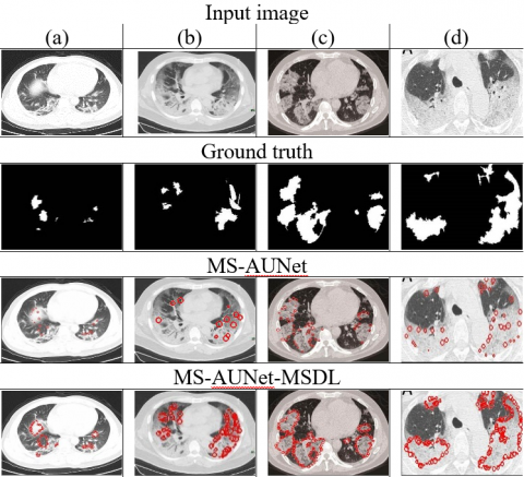
From Figure 4, it is observed that the trained MS-AUNet-MSDL can provide an accurate segmentation result when it segments infected tissues in small edge regions from the chest CT images. With the use of SDeepNet in marginal space and ASM, it can be viewed that the MS-AUNet-MSDL improves the segmentation results by learning shape abnormalities between normal and COVID-19 tissues in the lung boundaries. The MS-AUNet-MSDL can attain the output nearest to the ground truth and highly improve the COVID-19 segmentation performance.
Figure 4. Few examples of segmentation results for MS-AUNet-MSDL and MS-AUNet models on COVID-19 chest CT dataset
Table 1 presents the confusion matrices for the different DL-based segmentation models on the considered test CT images. This is used to calculate the performance of each model in terms of DS, HD, recall, precision, and RMSE.
Table 1. Confusion matrix for different DL-based segmentation models during testing phase
|
Models |
Detected Class |
|||
|
Actual |
Class |
0 |
1 |
|
|
Inf-Net [20] |
0 |
108 |
39 |
|
|
1 |
42 |
111 |
||
|
NormNet [21] |
Actual |
Class |
0 |
1 |
|
0 |
110 |
37 |
||
|
1 |
40 |
113 |
||
|
Anam-Net [22] |
Actual |
Class |
0 |
1 |
|
0 |
112 |
35 |
||
|
1 |
38 |
115 |
||
|
TSH-UNet [23] |
Actual |
Class |
0 |
1 |
|
0 |
114 |
33 |
||
|
1 |
36 |
117 |
||
|
SD-UNet [25] |
Actual |
Class |
0 |
1 |
|
0 |
115 |
31 |
||
|
1 |
35 |
119 |
||
|
Attention-RefNet [24] |
Actual |
Class |
0 |
1 |
|
0 |
117 |
30 |
||
|
1 |
33 |
120 |
||
|
MS-AUNet [14] |
Actual |
Class |
0 |
1 |
|
0 |
127 |
22 |
||
|
1 |
23 |
128 |
||
|
Proposed MS-AUNet-MSDL |
Actual |
Class |
0 |
1 |
|
0 |
132 |
18 |
||
|
1 |
18 |
132 |
||
*Note: 0 – Normal; 1 – COVID-19.
4.3 Dice Score (DS)
Its goal is to determine how closely categorization results and ground truth line up. The optimal solution has a higher DS.
Dice score $=\frac{2|P \cap \hat{P}|}{|P|+|\hat{P}|}$ (11)
Figure 5. Comparison of dice score for proposed and existing DL-based COVID-19 segmentation models
In Eq. (11), P refers to the pixel collection of the desired ROIs (COVID-19-infected tissues), $\hat{P}$ refers to the pixel collection of the infected ROIs segmented and categorized by the MS-AUNet-MSDL and $|\cdot|$ denotes the pixel quantity.
In Figure 5, the DS (in %) attained by various DL models used for lung CT image segmentation for COVID-19 diagnosis. It scrutinizes that the DS of MS-AUNet-MSDL is 18.18% greater than the Inf-Net, 16.04% greater than the NormNet, 13.83% greater than the Anam-Net, 11.29% greater than the SD-UNet, 10.2% greater than the TSH-UNet, 8.46% greater than the Attention-RefNet, and 3.82% greater than the MS-AUNet models. Thus, it realizes that the MS-AUNet-MSDL model enhances the DS contrasted with all other models due to the localization of healthy and COVID-19-infected tissues in the ROIs from the lung CT images.
4.4 Hausdorff Distance (HD)
It calculates the difference between the identified results and the ground truth and serves as a representation of the segmentation error. The HD of the ideal result is lower.
$H D=\max (d(P, \hat{P}), d(\hat{P}, P))$ (12)
where $d(P, \hat{P})=\max _{p \in P}\left(\min _{\hat{p} \in P}\|p-\hat{p}\|\right)$ (13)
$d(\hat{P}, P)=\max _{\hat{p} \in P}\left(\min _{p \in P}\|\hat{p}-p\|\right)$ (14)
In Eqs. (12) and (14), p and $\hat{p}$ indicate the pixels in P and $\hat{P}$, correspondingly, $\|\cdot\|$ denotes the Euclidean distance.
Figure 6. Comparison of Hausdorff distance for proposed and existing DL-based COVID-19 segmentation models
Figure 6 displays the HD (in mm) obtained by a variety of DL-based segmentation models used for COVID-19 identification and diagnosis. It indicates that the HD of MS-AUNet-MSDL is 49.02% smaller than the Inf-Net, 47.37% smaller than the NormNet, 46.13% smaller than the Anam-Net, 44.29% smaller than the SD-UNet, 42.61% smaller than the TSH-UNet, 40.83% smaller than the Attention-RefNet, and 19.01% smaller than the MS-AUNet models because of localizing the COVID-19-infected tissues in the ROIs from the lung CT images.
4.5 Recall
It is computed as:
Recall $=\frac{|P \cap \hat{P}|}{|P|}$ (15)
Figure 7. Comparison of recall for proposed and existing DL-based COVID-19 segmentation models
Figure 7 illustrates the recall (in %) attained by various DL models used for lung CT image segmentation for COVID-19 diagnosis. It analyzes that the recall of MS-AUNet-MSDL is 20.38% higher than the Inf-Net, 18.44% higher than the NormNet, 16.56% higher than the Anam-Net, 14.43% higher than the SD-UNet, 12.82% higher than the TSH-UNet, 11.25% higher than the Attention-RefNet, and 3.53% higher than the MS-AUNet models. Thus, it realizes that the MS-AUNet-MSDL model increases the recall compared to the other existing models for segmenting and localizing the COVID-19-infected lung tissues in the CT images.
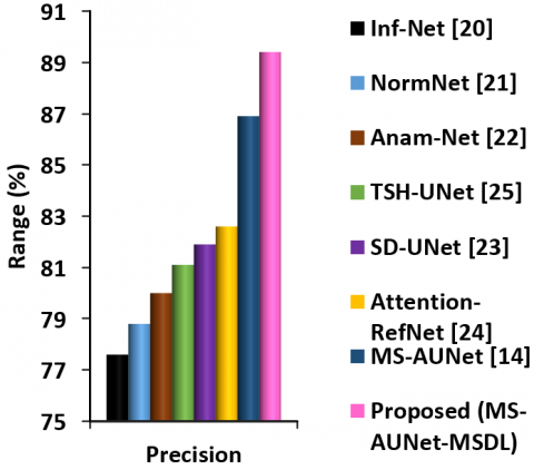
Figure 8. Comparison of precision for proposed and existing DL-based COVID-19 segmentation models
4.6 Precision
It is computed as:
Precision $=\frac{|P \cap \hat{P}|}{|\hat{P}|}$ (16)
Figure 8 illustrates the precision (in %) attained by various DL models used for lung CT image segmentation for COVID-19 diagnosis. It observes that the precision of MS-AUNet-MSDL is 15.21% higher than the Inf-Net, 13.45% higher than the NormNet, 11.75% higher than the Anam-Net, 10.23% higher than the SD-UNet, 9.16% higher than the TSH-UNet, 8.23% higher than the Attention-RefNet, and 2.88% higher than the MS-AUNet models. Thus, it realizes that the MS-AUNet-MSDL model increases the precision compared to the other models for segmenting and localizing the COVID-19-infected lung tissues in the CT images.
4.7 Root Mean Squared Error (RMSE)
It is employed to gauge how precise the segmentation is. It is calculated based on the square root of the MSE value as follows:
$R M S E=\sqrt{\frac{1}{N} \sum_i \sum_j\left(\hat{\delta}_{i j}-\delta_{i j}\right)^2} \times 100$ (17)
In Eq. (17), N indicates the sum quantity of images, $\hat{\mathcal{S}}$ indicates the segmented image, $\mathcal{S}$ indicates a real image and $i, j$ denote pixels in the images.
Figure 9. Comparison of RMSE for proposed and existing DL-based COVID-19 segmentation models
Figure 9 portrays the RMSE (in %) obtained by a variety of DL-based segmentation models used for COVID-19 identification and diagnosis. It indicates that the RMSE of MS-AUNet-MSDL is 20.29% less than the Inf-Net, 19.15% less than the NormNet, 17.99% less than the Anam-Net, 16.48% less than the SD-UNet, 15.24% less than the TSH-UNet, 13.64% less than the Attention-RefNet, and 9.16% less than the MS-AUNet models because of localizing the COVID-19-infected tissues in the ROIs from the lung CT images.
In this study, the MS-AUNet-MSDL model was developed to localize normal and COVID-19-infected tissues in the lung CT images. Initially, COVID-19 and normal chest CT images were obtained. After that, the MS-AUNet was used to segment the COVID-19-infected ROIs, which were further refined by the MSDL model. The MSDL using SDeepNet with MSL and ASM can predict the bounding boxes and shape abnormalities to accurately localize the healthy and COVID-19-infected tissues in the lung boundaries. The experimental outcomes of the MS-AUNet-MSDL model using the chest CT image dataset proved that it achieved 88% recall, 89.4% precision, and 89.7% DS, 11.42mm HD, and 22.8% RMSE contrasted with the existing variants of UNet models for COVID-19 detection.
Thus, this model can reduce the segmentation error and enhance the efficiency of COVID-19 diagnosis. It can be used by radiologists to detect COVID-19 infection from chest CT images and provide an appropriate diagnosis early to recover patients. However, more important discriminatory features were essential to categorize infection levels because quantifying infected tissues in the lung areas was not often achieve satisfactory solutions. Hence, future work will focus on classifying different stages of infection with the aid of more discriminative features from the chest CT images.
[1] Thakur, V., Bhola, S., Thakur, P., Patel, S.K.S., Kulshrestha, S., Ratho, R.K., Kumar, P. (2022). Waves and variants of SARS-CoV-2: Understanding the causes and effect of the COVID-19 catastrophe. Infection, 50: 309-325. https://doi.org/10.1007/s15010-021-01734-2
[2] Boraschi, P., Giugliano, L., Mercogliano, G., Donati, F., Romano, S. Neri, E. (2021). Abdominal and gastrointestinal manifestations in COVID-19 patients: Is imaging useful?. World Journal of Gastroenterology, 27(26): 4143-4159. https://doi.org/10.3748/wjg.v27.i26.4143
[3] Avila, R.S., Fain, S.B., Hatt, C., Armato III, S.G., Mulshine, J.L., Gierada, D., Sullivan, D.C. (2021). QIBA guidance: Computed tomography imaging for COVID-19 quantitative imaging applications. Clinical Imaging, 77: 151-157. https://doi.org/10.1016/j.clinimag.2021.02.017
[4] Alhasan, M., Hasaneen, M. (2021). Digital imaging, technologies and artificial intelligence applications during COVID-19 pandemic. Computerized Medical Imaging and Graphics, 91: 1-22. https://doi.org/10.1016/j.compmedimag.2021.101933
[5] Soomro, T.A., Zheng, L., Afifi, A.J., Ali, A., Yin, M., Gao, J. (2022). Artificial intelligence (AI) for medical imaging to combat coronavirus disease (COVID-19): A detailed review with direction for future research. Artificial Intelligence Review, 55: 1409-1439. https://doi.org/10.1007/s10462-021-09985-z
[6] Serena Low, W.C., Chuah, J.H., Tee, C.A.T., Anis, S., Shoaib, M.A., Faisal, A., Khalil, A., Lai, K.W. (2021). An overview of deep learning techniques on chest X-ray and CT scan identification of COVID-19. Computational and Mathematical Methods in Medicine, 2021: 1-17. https://doi.org/10.1155/2021/5528144
[7] Bouchareb, Y., Khaniabadi, P.M., Al Kindi, F., Al Dhuhli, H., Shiri, I., Zaidi, H., Rahmim, A. (2021). Artificial intelligence-driven assessment of radiological images for COVID-19. Computers in Biology and Medicine, 136: 1-17. https://doi.org/10.1016/j.compbiomed.2021.104665
[8] Huang, S., Yang, J., Fong, S., Zhao, Q. (2021). Artificial intelligence in the diagnosis of COVID-19: Challenges and perspectives. International Journal of Biological Sciences, 17(6): 1581-1587. https://doi.org/10.7150/ijbs.58855
[9] Fung, D.L., Liu, Q., Zammit, J., Leung, C.K.S., Hu, P. (2021). Self-supervised deep learning model for COVID-19 lung CT image segmentation highlighting putative causal relationship among age, underlying disease and COVID-19. Journal of Translational Medicine, 19(1): 1-18. https://doi.org/10.1186/s12967-021-02992-2
[10] Voulodimos, A., Protopapadakis, E., Katsamenis, I., Doulamis, A., Doulamis, N. (2021). A few-shot u-net deep learning model for COVID-19 infected area segmentation in CT images. Sensors, 21(6): 1-22. https://doi.org/10.3390/s21062215
[11] Ortiz, A., Trivedi, A., Desbiens, J., Blazes, M., Robinson, C., Gupta, S., Ferres, J.M.L. (2022). Effective deep learning approaches for predicting COVID-19 outcomes from chest computed tomography volumes. Scientific Reports, 12(1): 1-10. https://doi.org/10.1038/s41598-022-05532-0
[12] Shan, F., Gao, Y., Wang, J., Shi, W., Shi, N., Han, M., Shi, Y. (2021). Abnormal lung quantification in chest CT images of COVID‐19 patients with deep learning and its application to severity prediction. Medical Physics, 48(4): 1633-1645. https://doi.org/10.1002/mp.14609
[13] Yan, C., Wang, L., Lin, J., Xu, J., Zhang, T., Qi, J., Lambin, P.A. (2021). Fully automatic artificial intelligence–based CT image analysis system for accurate detection, diagnosis, and quantitative severity evaluation of pulmonary tuberculosis. European Radiology, 32(4): 2188-2199. https://doi.org/10.1007/s00330-021-08365-z
[14] Zhou, T., Canu, S., Ruan, S. (2021). Automatic COVID‐19 CT segmentation using U‐Net integrated spatial and channel attention mechanism. International Journal of Imaging Systems and Technology, 31(1): 16-27. https://doi.org/10.1002/ima.22527
[15] Enshaei, N., Oikonomou, A., Rafiee, M.J., Afshar, P., Heidarian, S., Mohammadi, A., Naderkhani, F. (2022). COVID-rate: An automated framework for segmentation of COVID-19 lesions from chest CT images. Scientific Reports, 12(1): 1-18. https://doi.org/10.1038/s41598-022-06854-9
[16] Yan, Q., Wang, B., Gong, D., Luo, C., Zhao, W., Shen, J., You, Z. (2021). COVID-19 chest CT image segmentation network by multi-scale fusion and enhancement operations. IEEE Transactions on Big Data, 7(1): 13-24. https://doi.org/10.1109/TBDATA.2021.3056564
[17] Polat, H. (2022). Multi-task semantic segmentation of CT images for COVID-19 infections using DeepLabV3+ based on dilated residual network. Physical and Engineering Sciences in Medicine, 45: 443-455. https://doi.org/10.1007/s13246-022-01110-w
[18] Li, C., Dong, L., Dou, Q., Lin, F., Zhang, K., Feng, Z., Heng, P.A. (2021). Self-ensembling co-training framework for semi-supervised COVID-19 CT segmentation. IEEE Journal of Biomedical and Health Informatics, 25(11): 4140-4151. https://doi.org/10.1109/JBHI.2021.3103646
[19] Yao, H.Y., Wan, W.G., Li, X. (2022). A deep adversarial model for segmentation-assisted COVID-19 diagnosis using CT images. EURASIP Journal on Advances in Signal Processing, 10: 1-17. https://doi.org/10.1186/s13634-022-00842-x
[20] Fan, D.P., Zhou, T., Ji, G.P., Zhou, Y., Chen, G., Fu, H., Shao, L. (2021). Inf-net: Automatic COVID-19 lung infection segmentation from CT images. IEEE Transactions on Medical Imaging, 39(8): 2626-2637. https://doi.org/10.1109/TMI.2020.2996645
[21] Yao, Q., Xiao, L., Liu, P., Zhou, S.K. (2021). Label-free segmentation of COVID-19 lesions in lung CT. IEEE Transactions on Medical Imaging, 40(10): 2808-2819. https://doi.org/10.1109/tmi.2021.3066161
[22] Paluru, N., Dayal, A., Jenssen, H.B., Sakinis, T., Cenkeramaddi, L.R., Prakash, J., Yalavarthy, P.K. (2021). Anam-Net: Anamorphic depth embedding-based lightweight CNN for segmentation of anomalies in COVID-19 chest CT images. IEEE Transactions on Neural Networks and Learning Systems, 32(3): 932-946. https://doi.org/10.1109/TNNLS.2021.3054746
[23] Shang, Y., Wei, Z., Hui, H., Li, X., Li, L., Yu, Y., Zha, Y. (2022). Two-stage hybrid network for segmentation of COVID-19 pneumonia lesions in CT images: A multicenter study. Medical & Biological Engineering & Computing, 60(9): 2721-2736. https://doi.org/10.1007/s11517-022-02619-8
[24] Kitrungrotsakul, T., Chen, Q., Wu, H., Iwamoto, Y., Hu, H., Zhu, W., Chen, Y.W. (2021). Attention-RefNet: Interactive attention refinement network for infected area segmentation of COVID-19. IEEE Journal of Biomedical and Health Informatics, 25(7): 2363-2373. https://doi.org/10.1109/JBHI.2021.3082527
[25] Yin, S., Deng, H., Xu, Z., Zhu, Q., Cheng, J. (2022). SD-UNet: a novel segmentation framework for CT images of lung infections. Electronics, 11(1): 1-19. https://doi.org/10.3390/electronics11010130
[26] Al-Zyoud, W., Erekat, D., Saraiji, R. (2023). COVID-19 chest X-ray image analysis by threshold-based segmentation. Heliyon, 9(3): 1-13. https://doi.org/10.1016/j.heliyon.2023.e14453
[27] Niu, S., Liu, M., Liu, Y., Wang, J., Song, H. (2021). Distant domain transfer learning for medical imaging. IEEE Journal of Biomedical and Health Informatics, 25(10): 3784-3793. https://doi.org/10.1109/JBHI.2021.3051470
[28] Gopatoti, A., Vijayalakshmi, P. (2022). Optimized chest X-ray image semantic segmentation networks for COVID-19 early detection. Journal of X-Ray Science and Technology, 30(3): 491-512. https://doi.org/10.3233/XST-211113
[29] Degerli, A., Ahishali, M., Yamac, M., Kiranyaz, S., Chowdhury, M.E., Hameed, K., Gabbouj, M. (2021). COVID-19 infection map generation and detection from chest X-ray images. Health Information Science and Systems, 9: 1-16. https://doi.org/10.1007/s13755-021-00146-8
[30] Zhang, P., Zhong, Y., Deng, Y., Tang, X., Li, X. (2020). DRR4Covid: Learning automated COVID-19 infection segmentation from digitally reconstructed radiographs. IEEE Access, 8: 207736-207757. https://doi.org/10.1109/ACCESS.2020.3038279
[31] Abdulah, H., Huber, B., Abdallah, H., Palese, L.L., Soltanian-Zadeh, H., Gatti, D.L. (2022). A hybrid pipeline for Covid-19 screening incorporating lungs segmentation and wavelet based preprocessing of chest X-rays. MedRxiv, 1-12. https://doi.org/10.1101/2022.03.13.22272311
[32] Zheng, Y., Barbu, A., Georgescu, B., Scheuering, M., Comaniciu, D. (2008). Four-chamber heart modeling and automatic segmentation for 3-D cardiac CT volumes using marginal space learning and steerable features. IEEE Transactions on Medical Imaging, 27(11): 1668-1681. https://doi.org/10.1109/TMI.2008.2004421
[33] Cootes, T., Baldock, E.R., Graham, J. (2000). An introduction to active shape models. Image Processing and Analysis, 328: 223-248.
[34] Radiopaedia-COVID-19 CT Cases-2020 dataset. http://www.radiopaedia.org.