Haritha Venkata Sai Lakshmi Inamanamelluri![]() | Venkateswara Rao Pulipati
| Venkateswara Rao Pulipati![]() | Nrusingha Charan Pradhan
| Nrusingha Charan Pradhan![]() | Phanikanth Chintamaneni
| Phanikanth Chintamaneni![]() | Manohar Manur
| Manohar Manur![]() | Ramesh Vatambeti*
| Ramesh Vatambeti*![]()
© 2023 IIETA. This article is published by IIETA and is licensed under the CC BY 4.0 license (http://creativecommons.org/licenses/by/4.0/).
OPEN ACCESS
A yellowing of the skin and eyes, called jaundice, is the consequence of an abnormally high bilirubin concentration in the blood. All across the world, both newborns and adults are afflicted by this illness. Jaundice is common in new-borns because their undeveloped livers have an imbalanced metabolic rate. Kernicterus is caused by a delay in detecting jaundice in a newborn, which can lead to other complications. The degree to which a newborn is affected by jaundice depends in large part on the mitotic count. Nonetheless, a promising tool is early diagnosis using AI-based applications. It is straightforward to implement, does not require any special skills, and comes at a minimal cost. The demand for AI in healthcare has led to the realisation that it may have practical applications in the medical industry. Using a deep learning algorithm, we created a method to categorise jaundice cases. In this study, we suggest using the binary spring search procedure (BSSA) to identify features and the XGBoost classifier to grade histopathology images automatically for mitotic activity. This investigation employs real-time and benchmark datasets, in addition to targeted methods, for identifying jaundice in infants. Evidence suggests that feature quality can have a negative effect on classification accuracy. Furthermore, a bottleneck in classification performance may emerge from compressing the classification approach for unique key attributes. Therefore, it is necessary to discover relevant features to use in classifier training. This can be achieved by integrating a feature selection strategy with a classification classical. Important findings from this study included the use of image processing methods in predicting neonatal hyperbilirubinemia. Image processing involves converting photos from analogue to digital form in order to edit them. Medical image processing aims to acquire data that can be used in the detection, diagnosis, monitoring, and treatment of disease. Newburn jaundice detection accuracy can be verified using image datasets. As opposed to more traditional methods, it produces more precise, timely, and cost-effective outcomes. Common performance metrics such as accuracy, sensitivity, and specificity were also predictive.
artificial intelligence, XGBoost classifier, new-born jaundice detection, binary spring search algorithm, neonatal hyperbilirubinemia
Most occurrences of jaundice in neonates are caused by the disintegration of cells, which release hematoidin into the blood, and the inability of the liver to adequately metabolise the bilirubin and make it available for elimination in the urine. High levels of hematoidin cause a xanthous staining of the whites of a new-born’s skin; symptoms include drowsiness and difficulty eating; consequences include convulsions, cerebral palsy, and kernicterus [1]. Pathologic jaundice is diagnosed in babies who are on their first day of life and have been present for more than two weeks, or if the newborn appears ill. It is common for neonates to acquire jaundice due to two causes [2]. To begin, the liver's hence foetal haemoglobin is degraded and replaced with adult haemoglobin, and bilirubin is eliminated as quickly as in an adult. Jaundice is caused by an excess of bilirubin in the blood, a condition known medically as hyperbilirubinemia. Second, if the neonatal jaundice does not improve with simple causes of liver disease in children, other options should be considered. These conditions include biliary atresia, Progressive familial deficiency, and others. Persistent neonatal jaundice is a medical emergency that must be treated right away [3].
Jaundice is caused by hyperbilirubinemia, which occurs in about 60% of babies and nearly 100% of preterm infants [4]. Jaundice is a somewhat common but usually harmless illness in neonates. Newborns aren't in danger of developing kernicterus unless the condition is misdiagnosed or treated late [5]. A chronic form of bilirubin encephalopathy known as kernicterus arises when bilirubin accumulates in the brain, causing irreparable damage [6]. Newborns at risk for developing must be correctly identified so that they can receive therapy as soon as possible. Therefore, protecting the baby from potentially harmful bilirubin levels is a top priority for doctors [7]. The risk of neonatal jaundice is currently evaluated using age-specific monograms that also factor in serum or other risk variables [8]. Studies have shown that there is a growing comeback, despite the fact that multiple methods are used to estimate the risk of developing brand-new hyperbilirubinemia [9].
Early diagnosis of jaundice in neonates and the related reduction in complications can be aided by knowledge of modifiable risk factors and the severity of the disease. There has been a rise in the number of babies being sent home from the hospital within the first 48 hours of life [10], and with such a brief postnatal hospital stay, jaundice may not have had time to manifest. Since many babies in Nigeria arrive at hospitals late with kernicterus, the country's neonatal mortality rate was 48 per 1,000 live births; an estimated 700 new-born’s died daily, totaling 284,000 deaths in a single year [11]. Neonatal hyperbilirubinemia is preventable, but only with prompt medical attention [12]. Parents should be able to spot neonatal bitterness and seek medical assistance for it immediately so that they can be discharged from the hospital sooner.
Data mining is one of the newest areas of science. It uses a wide range of statistical methods, ways to store data, AI tools, and pattern recognition, which is a branch of machine learning. Data mining, the application of statistical methods and AI to database management, is based on the ability to discover patterns and relations within massive datasets, which allows for the creation of models capable of assigning the class label to previously unlabeled cases [13]. Thus, data mining methods have been successfully implemented in many categorization problems [14]. Data mining's ability to unearth previously unsuspected connections has the potential to revolutionise our understanding of many medical conditions and motivate new studies in a wide range of scientific subfields. Data mining has helped the medical field thanks to the extremely high accuracy of the produced models [15]. Data mining has been shown to significantly improve the consequences achieved with existing approaches and contribute to new discoveries in several fields of medicine [16].
With the rise of big data and the advancement of computational control, machine learning techniques have emerged as a driving force in medical data analytics and knowledge discovery [17]. The need to apply machine learning algorithms to Big Data in order to uncover useful patterns has grown as the volume of patient data kept in healthcare databases has increased. Based on knowledge of preventable risk issues, this study employs machine learning to create a perfect organisation for the degree of jaundice in neonates. So, this paper focuses on creating a predictive model for the primary diagnosis of bitterness in newborns.
The contribution of the paper is given below:
The paper is organised as shadows: The associated work is described in Section 2. In the third section, we introduce the XGBoost algorithm we propose. In Section 4, we compare and contrast the proposed model to some commonly used validation methods. The study's conclusion and directions for future investigation are presented in Section 5.
Sreedha et al. [18] have focused on looking at the sclera as a way to find out if someone has jaundice. In the past, all efforts were based on getting data from hospitals, and there isn't a public dataset for analysing jaundice. Inadequate access to information is a key problem in the medical field. Insufficient data leads to inaccurate predictions in AI research. Although research in this field has progressed, past efforts have not focused on expanding the size of the dataset. In this study, we use the capabilities of the generative adversarial network (GAN) to address the problem of scarce medical data. This research presents a novel method for reliably gauging the severity of jaundice from the degree to which the sclera has turned yellow. The method is a mixture of computer vision and traditional machine learning. This work takes into account the sensitive nature of medical data and the difficulties posed by the scarcity of available datasets.
An intervention like the one recommended by Kalbande et al. [19] would be simple to implement, wouldn't require much money, and wouldn't put patients at risk. The potential utility of (AI) in the medical industry has been increasingly acknowledged in light of rising demand for AI in this sector. Using a deep learning algorithm, we created a method to categorise jaundice cases. To forecast jaundice from a picture of jaundiced eyes, we employed ResNet50 and masked the RCNN. With respect to eyes, our dataset includes 98 pictures of eyes with jaundice and 50 pictures of healthy eyes. Images of eyes affected by jaundice can be successfully segmented and classified using the Mask-RCNN model. According to the experiment results, the Mask-RCNN Deep Learning model outperforms ResNet50.
The research conducted by Samanta et al. [20] uses real-time and benchmark datasets, in addition to specialised methods, to identify neonatal jaundice. Evidence suggests that feature quality can have a negative effect on classification accuracy. Furthermore, a bottleneck in classification performance may emerge from compressing the classification approach for unique key attributes. Therefore, it is necessary to discover relevant features to use in classifier training. This can be achieved by integrating a feature selection strategy with a classification model. Important findings from this study included the use of image processing methods in predicting neonatal hyperbilirubinemia. In order to edit photos, image processing involves converting them from an analogue form to a digital one. Medical image processing aims to acquire data that can be used in the detection, diagnosis, monitoring, and treatment of disease. New-born jaundice detection accuracy can be verified using image datasets. As opposed to more traditional methods, it produces more precise, timely, and cost-effective outcomes. Common measures of performance, such as accuracy, sensitivity, and specificity, also showed predictive value.
To better facilitate the use of non-invasive technologies for the classification of neonatal jaundice, Hardalac et al. [21] have designed a transportable support system for hospital staff and medical personnel in outlying areas. As part of our research, we want to create an algorithm that can run on a mobile device, thereby drastically reducing the processing cost. As such, we develop a cheap strategy for finding the most important parameters by a combination of a regression model with numerous inputs and a correlation technique. The suggested method has the benefit of estimating bilirubin with the use of a straightforward regression curve. The low price is due to the use of a straightforward regression curve in place of the complex mathematical processes required by morphological image processing techniques for non-invasive jaundice prediction. There were a total of 196 participants in the study; 61 had moderate to severe jaundice, 95 had mild jaundice, and the remaining 40 served as test subjects. In this study, 40 test subjects were used to determine that the created algorithm has a two-group classification accuracy of 92.5%.
Wang et al. [22] present a new method for multi-class recognition of jaundice that can distinguish between occult jaundice, overt jaundice, and normal controls. Initial steps include creating and training a region annotation network to suggest potential eyes. Therefore, it is proposed to train a high-performance jaundice recognizer using topic photographs to identify them using their contextual knowledge, localization qualities, and globalisation traits. Finally, a common convolutional layer is used to bring together the two networks. When compared to a human expert, the structured model performed significantly better in performance evaluations (categorical accuracy for mean 91.38 percent). In comparison to the state-of-the-art convolutional neural network, our study achieved superior results (mean 95.33% on the testing subset, and 96.85% and 90.06% on the training and validation subsets, respectively). An improvement in performance, as compared to that of doctors, is achieved by using the proposed network. This research substantiates our concept as a viable means towards the eventual implementation of a powerful instrument for multi-class detection of jaundice in clinical settings.
There is evidence that the disease investigated by Kumar et al. [23] can cause brain injury and the resulting condition of kernicterus, which is marked by involuntary, repetitive movements, an abnormal fixation on the ceiling, and diminished hearing. Therefore, early diagnosis and treatment can reduce or eliminate consequences. Therefore, we have looked into how different researchers have gone about utilising various forms of AI to spot jaundice in new-borns. The examination we conducted of the various AI methods allowed us to draw certain conclusions, which we will now share. Both their successes and failures in this area were detailed in the study.
A highly accurate model for predicting jaundice has been developed by Sussma et al. [24]. This model can be used to any data set providing information on potential causes of jaundice. other components of a standard dataset are gathered. We employ PCA and factor analysis to isolate the most relevant and actionable variables in the jaundice diagnosis process. To improve the accuracy of the jaundice prediction, the dataset is trained using supervised learning models.
3.1 Skin detection
Colour space, model, and classification technique all affect how well skin detection works. Skin detection is a critical but time-consuming task that necessitates careful consideration of colour spaces before proceeding. These studies employ a wide variety of colour spaces, from the familiar RGB model to the more experimental YUV and YCbCr colour spaces [25, 26]. The RGB colour model is widely used to represent colour images in a variety of settings. For real-time skin identification, YUV or YCbCr colour spaces are frequently utilised, and the transition from YUV to RGB is linear. Y stands for the luma portion of the hue. Luma is a measurement of how brilliant a colour is. This is a reference to how bright the colour is. This part is designed to work better with the human visual system. Chroma has a blue component (Cb) and a red component (Cr). When compared to green," Cb is the blue component," while "Cr is the red component," as the definition puts it. The human visual system has lower sensitivity to these factors. In this dataset, we provide images of new-born infants with and without jaundice.
Through the process of this study, we transform the infant's input image from RGB to grayscale and then from grayscale to binary. Images with the skin's surface modified have the relevant parts cut out using a region of interest (ROI). After the piece was cut out, the hybrid median filter was used to get rid of any background noise that was still there. To make a classification method for jaundice, you have to build mathematical proofs and cut down on the amount of data used to classify an input signal. These mathematical models of motion can be thought of as a reduction of the space occupied by a multidimensional space into which various input signals have been mapped. This process of reducing the number of dimensions is known as "feature extraction." Finally, the extracted feature set should only contain the most crucial information from the original signal.
3.2 Pre-processing median
The median of the candidate region is the grey level value found exactly in the middle of the ordered list of grey level values.
$S D=\sqrt{\frac{1}{N-1} \sum_{i=1}^N\left(x_i-\bar{x}\right)^2}$ (1)
Images need to be denoised before being processed since the presence of sounds reduces the detecting system's effectiveness. Here, we denoise the raw infant image using the hybrid median filtering algorithm.
3.3 Feature selection using BSSA
Discrete-time optimisation of any issue is possible with the spring search algorithm, which is based on the spring force laws. The spring force law is used to make it easier for people involved in the optimisation process to talk to each other. In general, the suggested optimisation approach can be applied to any optimisation problem where the solution exists. The objective functions are used to calculate the spring stiffness coefficients.
The spring force law, often known as Hooke's law, is represented by Eq. (2). Within a specific allowance for length change, nearly all springs behave according to this law.
$F_s=-k x$ (2)
where, k is the constant of the spring force, x is the degree of expansion or reduction, and F s is the force exerted by the spring. The two stages of SSA are as follows: Step 1: Establishing a simulated system in the issue area that uses discrete time, setting initial positions for objects, enforcing rules, and fine-tuning parameters; Step 2: Performing discrete-time iterations until termination requirements are fulfilled.
3.3.1 System development, implementing laws and tuning strictures
The initial step is establishing the system's space. Each point in the search space, a multi-dimensional coordinate system, represents a possible answer to the problem at hand. Each object in a set of searching operators is connected to every other object in the set via springs. In the search space, each object has a location, and the springs attached to it have stiffness coefficients. Each spring's stiffness coefficient is adjusted in accordance with the fitness values of the two nodes. In SSA, the laws of motion and the spring force law regulate the system.
Reflect a system which contains of m objects; the site of each object represents a point in the space and a solution to the tricky. The subsequent phrase displays the location of the ith object:
$X_i=\left(x_i^1, \ldots, x_i^d, \ldots, x_i^n\right)$ for $i=1,2, \ldots, m$ (3)
where, x id is the location along the ith item's dth dimension. All objects are initially scattered around the search area in the problem. Depending on the forces applied to each other by the springs, these objects are gravitating towards equilibrium (the optimal solution). The spring stiffness coefficients are calculated using the following equation.
$K_{i, j}=K_{\max }\left|F_n^i-F_n^i\right| \max \left(F_n^i, F_n^j\right)$ (4)
where, Fni and Fnj are the normalised objective functions of the objects I and j, K (i,j) is the stiffness coefficient of the spring positioned among objects I and j, K max is the extreme value of stiffness springs and stated based on the optimization problem. Following are some expressions that are used to normalise the objective functions:
$F_n^{\prime i}=\frac{f_{o b j}^i}{\min \left(f_{o b j}\right)}$ (5)
$F_n^i=\frac{\min \left(F_n^{\prime i}\right)}{F_n^{\prime i}}$ (6)
where, f obj is the value of the impartial function for the object iteration I and f obji is the value of the objective function for the object iteration i+1. If we define an axis for each dimension of an m-dimensional optimization problem, we can find out how each variable is projected onto each axis. By comparing, the stable points on each axis are located on the left and right sides of the object. Stable points for a given object are simply locations where it has a higher fitness relative to other objects. So, each object experiences a sum of two forces along each axis. The formulations for the forces acting to the right and left of object j in dimension d are as follows:
$F_{\text {total }_R}^{j, d}=\sum_{i=1}^{n_R^d} K_{i, j} x_{i, j}^d$ (7)
$F_{\text {total }_L}^{j, d}=\sum_{l=1}^{n_L^d} K_{l, j} x_{i, j}^d$ (8)
where, K (i,j) and K (i,j) are the initial and final velocities, respectively, and F (total R)(j,d) and F (total L)(j,d) are the resulting forces on the right and left sides of object j in dimension d, the number of stable points on sides of object j in dimension d, and the distances between object j and the stable points on sides of object j in (l,j) The following are the outcomes of applying Hooke's law in dimension d.
$d X_R^{j, d}=\frac{F_{\text {total }\,_R}^{j, d}}{K_{\text {equal }\,_R}^j}$ (9)
$d X_L^{j, d}=\frac{F_{\text {total }\,_L}^{j, d}}{K_{\text {equal }\,_L}^j}$ (10)
where, rightward translation (dX R(j,d)) and leftward translation (dX L(j,d)) denote the translation of j to the right and left, correspondingly, in d. Therefore, we can calculate the resulting translation of item j in space dimension d by:
$d X^{j, d}=d X_R^{j, d}+d X_L^{j, d}$ (11)
where, the value may be either positive or negative. Therefore, the following phrase can be used to quickly get the current coordinates of Object j in Dimension d:
$X^{j, d}=X_0^{j, d}+r_1 \times d X^{j, d}$ (12)
For the sake of keeping the algorithm's random search behaviour intact, where X 0(j,d) is the preceding position of object j in dimension d, and r 1 is a uniformly distributed chance sum in the range [0,1].
3.3.2 Repetition and updating parameters
In the first phase of the search process, the positions of all objects are initially generated at random. Each object's updated position is calculated at each iteration using Eqns. (4)-(11) and its fitness value. Each iteration requires a change to a system parameter, the stiffness coefficients of the springs, according to Eq. (4). The optimization problem determines the stopping criteria, which may be the maximum sum of iterations. Here is a quick rundown of how the spring search algorithm works:
|
1. Defining the search space and initialization. 2. Initial positioning of objects. 3. Assessment and normalizing the fitness value of objects. 4. Updating the stiffness coefficients of the springs. 5. Formation of the spring force laws for each object. 6. Calculation of the displacement of each object. 7. Updating the position of each object. 8. Repeating stages 3-7 until the termination criteria are satisfied. 9. Select the object with the highest fitness value as the solution to the optimization problem. |
3.3.3 Binary spring search procedure
Particle motion in a discrete search space can be applied with a binary formulation. Think of a hype-cube, the corners of which have coordinates that are a sequence of ones and zeroes. It is pointed out that there is a solution to the problem in each of the hyper-vertices. cube's In order to conduct a search in such a setting, the things being sought must "hype-cube hop" from one corner to another. Every particle's coordinate in discrete search space is either zero or one. Each particle is able to travel by switching the value of one or more dimensions between zero and one. To do this, we use a probability function to take into account the sum of displacement for each object in each dimension, and assume that the object moves somewhere along that dimension. Therefore, in the binary version of SSA, the term "dX(j,d)" refers not to the translation of object j in dimension d but rather to the probability that X(j,d) is either zero or one.
The updating mechanism, the formulas used to calculate the force applied to each object, and the amount of displacement each object experiences are all the same in the binary version of SSA as they are in the continuous version. For binary SSA, the probability function defined as dX(j,d) should be limited to the interval [0,1]. Because of this, the following expression is commonly used:
$S\left(d X^{j, d}(t)\right)=\left|\tanh \left(d X^{j, d}(t)\right)\right|$ (13)
The three-dimensional coordinates of an item are found by using the probability function as follows:
If $\operatorname{rand}<S\left(d X^{j, d}(t)\right)$ then,
$X^{j, d}(t+1)=$ complement $\left(X^{j, d}(t)\right)$ (14)
Else $X^{j, d}(t+1)=X^{j, d}(t)$.
The likelihood that item j will move in dimension d is given by the expression (14), and it increases as the value of dX(j,d) increases. In the interval [0, 1], rand is a uniformly distributed random number.
3.4 Proposed XGBoost algorithm
The data set is split. The training data is applied to the proposed XGBoost algorithm with BSSA model to classify the data. The test data will be tested using an already trained XGBoost model. Finally, it predicts jaundice disease accurately. Extreme Gradient Boosting (XGBoost) is an ensemble tree that follows a gradient descent structure to enhance the weak learners. It is a level by level additive modelling. Initially, XGBoost fits the data to the weak classifier. Later, it fits the data to another weak classifier for increasing the ith accuracy. The overall workflow is summarized as follows:
Let consider the input features DS and it is represented in Eq. (15).
$D S=b: c, \quad|D S|=n, b \in R^m, c \in R$ (15)
where, n is the sum of occurrences, m denotes the sum of features, and b and c denote the features and target variable, correspondingly. The dataset contains n = 125 instances and m = 5 features. The sum of the predicted scores in k trees are calculated using Eq. (16).
$\widehat{c_i}=\sum_{k=1}^K f_k\left(b_i\right), \quad f_k \in F$ (16)
where, $\widehat{c_i}$ indicates the instance in the kth boost, $b_i$ indicates ith instance of training set.
The value of kth tree is represented by $f_k\left(b_i\right)$ and all the values of decision tree is represented by F. The XGBoost reduces the lose function $L_{\mathrm{k}}$ and it is given Eq. (17).
$L_k=\sum_{i=1}^n L\left(\widehat{c_i}, c_i\right)$ (17)
XGBoost defines the learning rate and hyper parameter values and it is given in Table 1.
Table 1. Parameters of proposed classifier
|
Parameters |
Default values |
|
Nthread |
Max |
|
Minimum child weight |
1 |
|
Maximum Depth |
6 |
|
Γ |
0 |
|
Learning rate |
0.2 |
|
A |
0 |
|
A |
1 |
|
Number of trees to fit |
100 |
In XGBoost, the objective function considers the loss function and regularization term to choose predicate function. The Objective Function (OF) of XGBoost is given in Eq. (18).
$O F=\sum_{i=1}^n\left(\widehat{c}_i, c_i\right)+\sum_{i=1}^k R\left(f_i\right)$ (18)
where, L indicates the loss function, $\widehat{C_i}$ indicates predicted label and $c_i$ indicates actual label. R(f) indicates penalizing computing function in the training tree.
To define the complexity, we first define the tree function $f(b)$, which is given in Eq. (19).
$f(b)=w_q(b), w \in R^L, q: R^m \rightarrow\{1,2, \ldots L\}$ (19)
where, w indicates the leaf score of the tree, q indicates mapping function between data samples and corresponding leaf. The L indicates number of leaves in the tree.
The complexity of penalize model’s calculation is given in Eq. (20).
$R(f)=\gamma \times L+a(\|w\|)+\frac{1}{2} \times \lambda \times\|w\|^2$ (20)
where, λ and γ are constant values, each leaf value is represented by γ. $\|w\|$ indicates weight value of the tree.
The XGBoost follows an additive model which indicates the curve tree result with previous tree result. At t-th step, the Objective Function (OF) is calculated and it is given in Eq. (21).
$O F^{(T)}=\sum_{i=1}^n L\left(c_i, \hat{c}_i^t\right)+f_t\left(b_i\right)+R\left(f_t\right)+c$ (21)
where, $f_t$ indicates minimization of objective function and c is a constant.
Further, we compute the second order Taylor series and it is given in Eq. (22).
$O F^{(T)}=\sum_{i=1}^n\left[L\left(c_i, \hat{c}_i^{t-1}\right)+g_i \times f_t\left(b_i\right)\right.$$\left.+\frac{1}{2} \times h_i f_t^2\left(b_i\right)\right]+R\left(f_t\right)+c$ (22)
The calculation of $g_{\mathrm{i}}$ and $h_{\mathrm{i}}$ are given in Eqns. (23)-(24).
$g_i=\partial_{\hat{c}_i^{t-1}} L\left(c_i, \hat{c}_i^{t-1}\right)$ (23)
$h_i=\partial_{\hat{c}_i^{t-1}}{ }^2 L\left(c_i, \hat{c}_i^{t-1}\right)$ (24)
In order to remove constant, we obtain Eq. (12) by adding regularization term from Eq. (20).
$O F^{(T)}=\sum_{i=1}^n\left[g_i \times f_t\left(b_i\right)+\frac{1}{2} \times h_i f_t^2\left(b_i\right)\right]+\gamma^t$$+\alpha \times \sum_{j=1}^T w_i^2$ (25)
Finally, the XGBoost algorithm is selected good features and predicts the disease accurately. The overall XGBoost classification process is given in Algorithm 2.
|
Algorithm 2 Proposed XGBoost |
|
Input: Features from BSSA Output: Prediction of jaundice disease 1: Dataset is split into training, testing and validation set 2: sum of predicted tree is calculated using Eq. (16) 3: XGBoost loss function is calculated using Eq. (17). 4: Objective function calculation process $O F=\sum_{i=1}^n L\left(\hat{c}_i, c_i\right)+\sum_{i=1}^k R\left(f_i\right)$ 5: XGBoost tree construction is defined in Eq. (19). 6: The complexity of penalize model is calculated using Eq. (20). 7: Final tree construction process is calculated using Eq. (25). 8: The test set is matched with XGboost decision function 9: Prediction of jaundice diseases. |
The suggested procedure is run on a 2.30 GHz Intel(R) Core (TM) i5-2410M CPU with 16 GB of RAM using Matlab 2013a. Since baby jaundice can have long-term effects on mobility, it can be used as a case study to test how well the suggested model (BSSA-XGBoost) works. There are numerous unorganised locations where one can find information about jaundice. These preliminary tests relied on the testing data provided by the Kaggle dataset. All subsequent studies make use of the information collected for the new-born jaundice prediction research. This was done because it was easier to evaluate the system's precision by analysing multiple patients, particularly children. The second stage of the experiment was designed to determine how long a preictal state would need to last in order to adequately reveal the factors that underlie the onset of jaundice.
By eliminating noise and assessing key patterns in the images, the pre-processing phase enhances the data set for further analysis. In this experiment, we record and use data from multiple infant jaundice datasets, none of which are related to one another, to find the feature sets that maximise prediction accuracy. These evaluations show how well different classifiers perform and how closely they model state transition behaviour.
Visually, pre-processing activity in an input image is frequently easy to spot due to the jaundiced aspect of the image, which occurs because the colours of one set of data become more apparent as they go from the beginning to the conclusion of the image. This was a clear indication of how the foreseen forecasting mechanism functioned. An initial guess of whether the states were defined as jaundice or not was necessary for recognition. Matrix results from the proposed system are presented in Table 2.
Table 2. Confusion matrix
|
Confusion matrix |
Predicted |
||
|
Normal |
Jaundice |
||
|
Actual |
Normal |
63 |
4 |
|
Jaundice |
3 |
72 |
|
Table 2 gives examples of confusion matrix values that were used to create a prediction model for recognising the jaundice state based on the data collected from prior experiments. The aggregate amounts are broken out between the typical and jaundice-predicted ranges.
According to the formula (26), the proposed classification system's efficacy is measured by its sensitivity, specificity, accuracy, precision, and F1 score for anticipated and annotated outcomes (29).
Accuracy $=(T P+T N) /(T P+T N+F P+F N)$ (26)
Sensitivity $=T P /(T P+F N)$ (27)
Specificity $=T N /(T N+F P)$ (28)
$F 1$ score $=2\left(\frac{\text { Precision } * \text { Recall }}{\text { Precision }+ \text { Recall }}\right)$ (29)
Based on Table 3 values, the subsequent presentation assessments are measured and the proposed system is associated to the existing models. The existing models are focused on eye images or Kaggle images for adults, but the proposed model uses histopathological images for new-born babies. Therefore, generic machine learning techniques are considered for validation, which is implemented and results are averaged.
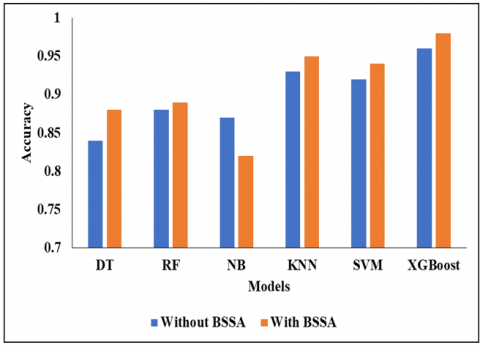
Table 3 shows the analysis of the proposed classifier without BSSA. In this analysis, we have used different classifiers such as DT, RF, NB, KNN, SVM, and XGBoost. Initially, the DT classifier reached an accuracy of 0.84%, a sensitivity of 0.55%, a specificity of 0.88%, the f-measure value of 0.70s such as DT, RF, NB, KNN, SVM, and XGBoost. Initially, the DT classifier reached an accuracy of 0.84%, a sensitivity of 0.55%, a specificity of 0.88%, the f-measure value of 0.70%, and finally, the FPR rate of 0.62%. Initially, the DT classifier reached an accuracy of 0.84%, a sensitivity of 0.55%, a specificity of 0.88%, the f-measure value of 0.70s such as DT, RF, NB, KNN, SVM, and XGBoost. Initially, the DT classifier reached an accuracy of 0.84%, a sensitivity of 0.55%, a specificity of 0.88%, the f-measure value of 0.70%, and finally, the FPR rate of 0.62%. Initially, the DT classifier reached an accuracy of 0.84%, a sensitivity of 0.55%, a specificity of 0.88%, the f-measure value of 0.70%, and finally, the FPR rate of 0.62%.
Table 3. Analysis of proposed classifier without BSSA
|
Classifier |
ACC |
SEN |
SPEC |
F-MEASURE |
FPR |
|
DT |
0.84 |
0.55 |
0.88 |
0.70 |
0.62 |
|
RF |
0.88 |
0.62 |
0.89 |
0.76 |
0.53 |
|
NB |
0.87 |
0.65 |
0.90 |
0.78 |
0.50 |
|
KNN |
0.93 |
0.75 |
0.94 |
0.85 |
0.49 |
|
SVM |
0.92 |
0.79 |
0.96 |
0.89 |
0.48 |
|
XGBoost |
0.96 |
0.91 |
0.97 |
0.95 |
0.47 |
Figure 1. Accuracy comparison
Figure 2. Sensitivity comparison
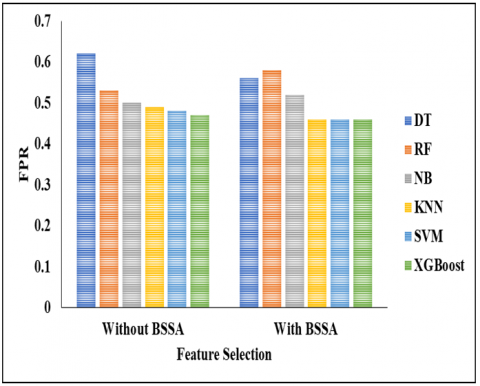
Initially, the RF classifier achieved an accuracy of 0.88%, sensitivity of 0.62%, specificity of 0.89%, f-measure value of 0.76%, and FPR rate of 0.53%. The NB classifier initially achieved an accuracy of 0.87%, sensitivity of 0.65%, specificity of 0.90%, and f-measure value of 0.78%, eventually achieving an FPR rate of 0.50%. Initially, the KNN classifier reached an accuracy of 0.93%, a sensitivity of 0.75%, a specificity of 0.94%, the f-measure value of 0.85 %, and finally the FPR rate of 0.49%. The SVM classifier initially achieved an accuracy of 0.92%, a sensitivity of 0.79%, a specificity of 0.96%, an f-measure value of 0.89%, and an FPR rate of 0.48%. Initially, the XGBoost classifier reached an accuracy of 0.96%, a sensitivity of 0.91%, a specificity of 0.97%, and an f-measure value of 0.95%, finally resulting in an FPR rate of 0.47%. In this comparison analysis, the proposed model achieved better results than the other compared methods. Accuracy comparison of classifers DT, RF, NB, KNN, SVM and XGBoost is shown in Figure 1. Figure 2 shows Sensitivity comparison.
Table 4 shows the analysis of the proposed classifier without BSSA. In this analysis, we used classifiers such as DT, RF, NB, KNN, SVM, and XGBoost. Figures 3, 4, and 5 show specificity comparisons, F-measure comparisons, and FPR comparisons of these classifiers. Initially, the DT classifier reached an accuracy of 0.88%, a sensitivity of 0.56%, a specificity of 0.90%, the f-measure value of 0.73%, and finally, the FPR rate of 0.56%. Initially, the DT classifier reached an accuracy of 0.88%, a sensitivity of 0.55%, a specificity of 0.88%, the f-measure value of 0.70 as DT, RF, NB, KNN, SVM and XGBoost classifier. Initially, the DT classifier reached an accuracy of 0.88%, a sensitivity of 0.56%, a specificity of 0.90%, the f-measure value of 0.73%, and finally, the FPR rate of 0.56%. Initially, the DT classifier reached an accuracy of 0.88%, a sensitivity of 0.55%, a specificity of 0.88%, the f-measure value of 0.70%, and finally the FPR rate of 0.62%. Initially, the RF classifier achieved an accuracy of 0.88%, a sensitivity of 0.62%, a specificity of 0.89%, an f-measure value of 0.76 %, and an FPR rate of 0.53%. Initially, the NB classifier achieved an accuracy of 0.82%, a sensitivity of 0.65%, a specificity of 0.70%, an f-measure value of 0.93%, and an FPR rate of 0.52%. Initially, the KNN classifier reached an accuracy of 0.95%, a sensitivity of 0.75%, a specificity of 0.94%, the f-measure value of 0.85%, and finally the FPR rate of 0.49%. The SVM classifier initially achieved an accuracy of 0.92%, a sensitivity of 0.79%, a specificity of 0.96%, an f-measure value of 0.89%, and an FPR rate of 0.48%. Initially, the XGBoost classifier reached an accuracy of 0.98%, a sensitivity of 0.96%, a specificity of 0.98%, and an f-measure value of 0.96%, finally reaching an FPR rate of 0.46%. In this comparison analysis, the proposed model achieved better results than the other compared methods.
Table 4. Analysis of proposed classifier with BSSA
|
Classifier |
ACC |
SEN |
SPEC |
F-MEASURE |
FPR |
|
DT |
0.88 |
0.56 |
0.90 |
0.73 |
0.56 |
|
RF |
0.89 |
0.66 |
0.91 |
0.80 |
0.58 |
|
NB |
0.82 |
0.70 |
0.93 |
0.83 |
0.52 |
|
KNN |
0.95 |
0.89 |
0.95 |
0.90 |
0.46 |
|
SVM |
0.94 |
0.89 |
0.97 |
0.93 |
0.46 |
|
XGBoost |
0.98 |
0.96 |
0.98 |
0.96 |
0.46 |
Figure 3. Specificity comparison
Figure 4. F-Measure comparison
Figure 5. FPR comparison
A dataset of images of the skin of new-born babies was used to construct a classification model for predicting the degree of value of factors. We used the historical dataset for training and testing, as well as the BSSA with XGBoost classifier, to create a classification model for the severity of neonatal jaundice. Classifier-based prediction models were trained using 10-fold cross-validation, and their efficacy was assessed. Researchers looked into which feature sets were the most effective overall. Numerous studies have reported the detection of illnesses in newborns, including jaundice, but have not succeeded in reliably removing the jaundice. Accuracy, specificity, and sensitivity of 98%, 98%, and 96%, respectively, are achieved by the suggested approach of automatic new-born jaundice identification in histopathological pictures and grading using the BSSA feature jaundice in infants. There are no limitations in this research work. Research on soft computing-based classifiers for high-dimensional databases is planned for the future.
[1] Damodaran, S.P., Srinivasan, V.K., Rajakani, K. (2019). Optimized and low-complexity power allocation and beamforming with full duplex in massive MIMO and small-cell networks. The Journal of Supercomputing, 75(1). https://link.springer.com/article/10.1007/s11227-018-2400-z
[2] Samanta, D., Karthikeyan, M., Banerjee, A., Inokawa, H. (2021). Tunable graphene nanopatch antenna design for on-chip integrated terahertz detector arrays with potential application in cancer imaging. Nanomedicine, 16(12): 1035-1047. https://doi.org/10.2217/nnm-2020-0386
[3] Mukkapati, N., Anbarasi, M.S. (2022). Brain tumor classification based on enhanced CNN model. Revue d'Intelligence Artificielle, 3(1): 125-130. https://doi.org/10.18280/ria.360114
[4] Khamparia, A., Singh, P. K., Rani, P., Samanta, D., Khanna, A., Bhushan, B. (2021). An internet of health things-driven deep learning framework for detection and classification of skin cancer using transfer learning. Transactions on Emerging Telecommunications Technologies, 32(7): e3963. http://dx.doi.org/10.1002/ett.3963
[5] Bactavatchalame, P., Rajakani, K. (2020). Compact broadband slot-based MIMO antenna array for vehicular environment. Microwave and Optical Technology Letters, 62(5): 2024-2032. http://dx.doi.org/10.1002/mop.32261
[6] Uma Maheswari, V., Aluvalu, R., Chennam, K.K. (2021). Application of machine learning algorithms for facial expression analysis. Machine Learning for Sustainable Development, 9(77). https://doi.org/10.1515/9783110702514-005
[7] Inamori, G., Kamoto, U., Nakamura, F., Isoda, Y., Uozumi, A., Matsuda, R., Shimamura, M., Okubo, Y., Ito, S., Ota, H. (2021). Neonatal wearable device for colorimetry-based real-time detection of jaundice with simultaneous sensing of vitals. Science Advances, 7(10): eabe3793. https://doi.org/10.1126/sciadv.abe3793
[8] S Srastika, N., Bhandary, N., Honnavalli, S. P., Eswaran, S. (2022). An enhanced malware detection approach using machine learning and feature selection. In 2022 3rd International Conference on Electronics and Sustainable Communication Systems (ICESC), pp. 909-914. https://doi.org/10.1109/ICESC54411.2022.9885509
[9] Hsu, W.Y., Cheng, H.C. (2021). A fast and effective system for detection of neonatal jaundice with a dynamic threshold white balance algorithm. Healthcare, 9(8): 1052. https://doi.org/10.3390/healthcare9081052
[10] Kasthuri, S., Jebaseeli, A.N. (2020). An efficient decision tree algorithm for analyzing the twitter sentiment analysis. Journal of Critical Reviews, 7(4): 1010-1018.
[11] Chakraborty, A., Goud, S., Shetty, V., Bhattacharyya, B. (2020). Neonatal jaundice detection system using CNN algorithm and image processing. International Journal of Electrical Engineering and Technology, 11(3): 248-264. http://dx.doi.org/10.34218/IJEET.11.3.2020.029
[12] Wagle, S.A., R, H. (2021). A deep learning-based approach in classification and validation of tomato leaf disease. Traitement du Signal, 38(3): 699-709. https://doi.org/10.18280/ts.380317
[13] Vatambeti, R., Mantena, S.V., Kiran, K.V.D., et al. (2023). Twitter sentiment analysis on online food services based on elephant herd optimization with hybrid deep learning technique. Cluster Computing. https://doi.org/10.1007/s10586-023-03970-7
[14] Sanshi, S., Pramodh Krishna, D., Vatambeti, R. (2022). Enhancing the communication of IoT using African Buffalo delay tolerant and risk packet jump approach. WSEAS Transactions on Information Science and Applications, 19: 193-201. http://dx.doi.org/10.37394/23209.2022.19.20
[15] Hashim, W., Alkhaled, M., Al-Naji, A. Al-Rayahi, I. (2021). A review on image processing based neonatal jaundice detection techniques. In 2021 7th International Conference on Contemporary Information Technology and Mathematics (ICCITM), pp. 213-218.
[16] Nandihal, P., Shetty S, V., Guha, T., Pareek, P.K. (2022). Glioma detection using improved artificial neural network in MRI images. In 2022 IEEE 2nd Mysore Sub Section International Conference (MysuruCon), pp. 1-9. https://doi.org/10.1109/MysuruCon55714.2022.9972712.
[17] Nihila, S., Rajalakshmi, T., Panda, S.S., Lhazay, N., Giri, G.D. (2021). Detection of jaundice in neonates using artificial intelligence. In Soft Computing: Theories and Applications: Proceedings of SoCTA 2020, 2: 431-443.
[18] Sreedha, B., Nair, P.R., Maity, R. (2023). Non-invasive early diagnosis of jaundice with computer vision. Procedia Computer Science, 218: 1321-1334. https://doi.org/10.1016/j.procs.2023.01.111
[19] Kalbande, D., Majumdar, A., Dorik, P., Prajapati, P., Deshpande, S. (2022). Deep learning approach for early diagnosis of Jaundice. In International Conference on Innovative Computing and Communications: Proceedings of ICICC 2022, 3: 387-395. http://dx.doi.org/10.1007/978-981-19-3679-1_30
[20] Samanta, D., Karthikeyan, M.P., Karuppiah, M., Parwani, D., Maheshwari, M., Shukla, P.K., Nuagah, S.J. (2021). Optimized tree strategy with principal component analysis using feature selection-based classification for newborn infant’s Jaundice symptoms. Journal of Healthcare Engineering, 2021: 9806011. https://doi.org/10.1155/2021/9806011
[21] Hardalac, F., Aydin, M., Kutbay, U.Ğ.U.R.H.A.N., Ayturan, K., Akyel, A., Çağlar, A., Hai, B., Mert, F. (2021). Classification of neonatal jaundice in mobile application with noninvasive imageprocessing methods. Turkish Journal of Electrical Engineering and Computer Sciences, 29(4): 2116-2126. http://dx.doi.org/10.3906/elk-2008-76
[22] Wang, Z., Xiao, Y., Weng, F., Li, X., Zhu, D., Lu, F., Liu, X., Hou, M., Meng, Y. (2021). R-JaunLab: automatic multi-class recognition of jaundice on photos of subjects with region annotation networks. Journal of Digital Imaging, 34: 337-350. https://doi.org/10.1007/s10278-021-00432-7
[23] Kumar, Y., Patel, N.P., Koul, A., Gupta, A. (2022). Early prediction of neonatal jaundice using artificial intelligence techniques. In 2022 2nd international conference on innovative practices in technology and management (ICIPTM), India, pp. 222-226. https://doi.org/10.1109/ICIPTM54933.2022.9753884
[24] Sussma, S., Nadu, T., Srivignesh, S., Kishore, V.S., Marimuthu, M. (2022). Jaundice prediction using machine learning approach. International Journal of Advance Research, Ideas and Innovations in Technology, 7(6).
[25] Vatambeti, R. Damera, V.K. (2022). Gait based person identification using deep learning model of generative adversarial network (GAN). Acadlore Transactions on AI and Machine Learning, 1(2): 90-100. https://doi.org/10.56578/ataiml010203
[26] Khare, V., Kumari, S. (2022). Performance comparison of three classifiers for fetal health classification based on cardiotocographic data. Acadlore Transactions on AI and Machine Learning, 1(1): 52-60. https://doi.org/10.56578/ataiml010107