Manish Kumar Mishra* | Ritesh Kumar Mishra
© 2022 IIETA. This article is published by IIETA and is licensed under the CC BY 4.0 license (http://creativecommons.org/licenses/by/4.0/).
OPEN ACCESS
In this paper, Hybrid satellite-terrestrial systems (HSTC) are preferred in dynamic type environments with high mobility of nodes due to the performance enhancement features in multiple relay-based selective decode-and-forward (DF) approach. Because of the satellite link, aerial satellite to destination and satellite to relay links, are not the same due to time-selective shadowed Rician fading. Time-selective Rician fading depends on parameters like the angle of elevation of the satellite, the terrestrial relay node, and the node destination links, considered to be distinctively time-selective Nakagami faded. Here, per-frame average symbol error rate (SER) and outage probability are derived in a closed-form expression with consideration of M-ary PSK modulated symbols transmission. After evaluation, it was detected that the system performance is significantly degraded due to the time-varying nature of the links (dynamic environment). After various simulations and calculations, it was established that the error rate of the HSTC is significantly low by increasing the elevation angle of the satellite on the relay point. The performance enhancement can be observed by enhancing the satellite angle at the destination node of user equipment.
hybrid satellite-terrestrial systems (HSTC), outage probability, symbol error rate (SER), decode and forward (DF), Nakagami-m fading channel
In conventional satellite communication systems, satellites coverage issues are major concern which can be rectify unto a certain level by adopting hybrid satellite-terrestrial systems. Coverage problem inside buildings and other shadowed regions like in the shade of any high height buildings or under the shade of mountains where line of sight (LOS) communication was not able to be established because of masking effect [1-3] is reduced by hybrid satellite-terrestrial systems. Due to this reason hybrid satellite-terrestrial systems have gained quite interest of research. This gives improved bandwidth utilization, increased reliability and enables higher data rate with less SER for broadcasting and navigation applications at less cost as compared to convention satellite systems. Masking effect is more effective at lower satellite elevation angles and it is also creating problem in outdoor environment scenario like in free space. If mobility is also considered in the real outdoor environment scenario, then mobility of the user equipment (UE) and cooperative user equipment’s working as relay nodes produces Doppler effect. Doppler effect causes time-selective fading [4-6], therefore worse the satellite to destination performance. The investigation of the outcome of node mobility and the associated time- selective fading connections on HSTC is summarized in Refs. [7-9]. Also explained, the HSTC, where the shadowing effect is also a concern while calculating the performance of the satellite-terrestrial link. Shankar et al. [10] demonstrated the precise HSTCN outage probability expression utilizing DF and the optimal relay selection technique. As work in [11, 12] described and analyze the SER and outage execution of a hybrid satellite-terrestrial cooperative system in different fading channels. Outage problem is major concern in all wireless systems where given information rate is not supported by channel due to variable channel capacity i.e. available information rate is less than the required threshold level. Even so, the description explained the amplify-and-forward (AF) method, where noise amplification takes place at the relay nodes [13-15]. The studies [16-18] focused on the SER of a hybrid satellite-terrestrial selective DF cooperative system and documented their findings following the Lauricella hypergeometric functions with finite sums. Both works [19, 20] used different approaches of cooperative network but do not include the effect of angle of elevations and also time-selectivity on the satellite to destination node fulfillment. The pairwise error probability analysis of spatial modulated (SM)-MIMO network in k-μ fading channel [21]. McKay et al. [22] have analyzed ergodic capacity and average SER accomplishment of a HSTC system with pre-defined fixed gain considering amplify-and-forward (AF) method. The satellite system's aerial and terrestrial connections anticipated experiencing shadowed Rician and Rayleigh fading in these sections. The same type of issues is considered and studied [23-25], in the presence of co-channel interference (CCI). Furthermore, various research has been conducted at dual-hop HSTC systems using either amplify-and-forward (AF) or constant decode-and-forward (DF) relaying approach at the relay node of the system, such as the studies [26-29]. Moreover, various performance merits of hybrid satellite– terrestrial relay networks under interference-limited scenarios, including OP, ASER, and ergodic capacity, have been investigated in Refs. [30]. Furthermore, none of the previous studies addressed considers temporal selectivity and its influence on the system's overall performance while utilizing the vigorous selective decode and forward cooperative approach.
This paper examines the performance of HSTC systems with the time-selected fading connections along with multiple relays and selective decode and forward collaboration. Besides, the satellite and terrestrial connections in a land mobile satellite network were, intended to be a conventional separate time-selective shadowed-Rician fading type, with variables dependent on the satellite angle of elevation. The angle of elevation of the satellite is an approach to performance optimization. The terrestrial links established between the relay node and the destination terminal are expected to be specific time-selective generalized Nakagami fading where delay-time spreads are relatively large. As the nature of the satellite and terrestrial links is time-varying, the performance of the end-to-end hybrid satellite-terrestrial communication system becomes noticeable decreases. In addition, the effect of elevation angles of a satellite is analyzed in this paper. Also, to mention, that by setting the correlation variable to unity, the outcome of the quasi-static channel, while using the stable terrestrial node can be generated more effectively.
The rest of this paper is arranged in the following manner. In Section II, the system model of HSTC network is introduced. The expression for outage probability is discussed in Section III. The expression for symbol error rate (SER) is discussed in Section IV. The simulation result is presented in Section V. Section VI contains the conclusions.
Taking into account, an HSTC system as shown in Figure 1 with selective decode and forward-based collaboration where the k terrestrial relay nodes work together with a hybrid satellite to selective re-transmit M-array PSK modulated satellite information to a target user equipment via orthogonal channel connections. Each relay node and the destination UE, handled as if, they were mobile at any speed in this research, which makes the connection between satellite to destination, relay to destination, and satellite to relay, time selective.
Figure 1. System model of the HSTC communication with non- static Terrestrial Node
In addition, unlike previous research [2, 3, 11], this study looks at a direct satellite-destination relationship as well as an elevation angle $\phi_{S D}$. HSTC is used, in the context of mass broadcasting and navigation due to its ability to provide satellite coverage inside buildings and other shadowed areas. The direct relationship between satellites and destinations is given in Eq. (1). The angle of elevation forming between satellite and relay r is represented as $\phi_{S R_{r}}$, here value of r=1,2,3....K. And when the two-phase network, taking into account, the received signals $z_{S D}[k]$ and $z_{S R_{r}}[k]$ at the end terminal and relay r respectively, by the transmitting signal x[K] from the satellite terminal in the kth period of signaling, $1 \leq k \leq N_{b}$, expressed as,
$z_{S D}[k]=\sqrt{\varphi_{0}} \hbar_{S D}[k] x[k]+\mu_{S D}[k]$ (1)
$z_{S R_{r}}[k]=\sqrt{\varphi_{0}} \hbar_{S R_{r}}[k] x[k]+\mu_{S R_{r}}[k]$ (2)
Here $1 \leq r \leq K$, $\varphi_{o}$ means source transmitted power and $\hbar_{S D}[k]$, $\hbar_{S R_{r}}[k]$ are the value, time-varying channel coefficients for the hybrid satellite to end terminal and satellite to relay r connection respectively. In addition, multiple relays are deployed in the second phase of the process, and only send the symbol data to the end terminal if the value of the decoding SNR exceeds a preset threshold value [5, 8]. The received signal $z_{R_{r} D\lceil k\rceil}$ at the end terminal corresponding to relay transmission is expressed as:
$z_{R_{r} D}[k]=\sqrt{\varphi_{r}} \hbar_{R_{r} D}[k] x[k]+\mu_{R_{r} D}[k]$ (3)
where, $z_{R_{r} D\lceil k\rceil}$ is the channel coefficient of the time-varying r -relay to destination connection and $\varphi_{o}$ represents the power transferred by the r relay. The additive white noise components $\mu_{S D}[k]$, $\mu_{R_{r} D}[k]$ and $\mu_{S R_{r}}[k]$ at the end terminal, relay r, and above may be expressed as zero mean Gaussian random variables having variances $\eta_{o}$.
As the connection is time selective, obtaining the instantaneous CSI for each signaling period might be challenging. As a result, the channel coefficients $\hbar_{S R_{r}}[L]$, $\hbar_{S D}[L]$ and $\hbar_{R_{r} D}[L]$ at the $r^{t h}$ relay and user equipment’s are expected to be properly calculated [17, 18]. Each frame's $L^{t h}$ signaling instant is used once, and then are used to find each symbol x[K], $1 \leq k \leq N_{b}$, in the matching frame with the length $N_{b}$. As the receiver tracking loop is not able to predict the gain of the channels in signaling period k owing to the much greater pilot overhead required [4], this is a reasonable consideration in conventional wireless communication systems. It's also worth noting that, with the right L, the model may support both a preamble and a mid-amble for channel estimation. Here we are utilizing the first-order autoregressive (AR1) process [19] to describe the time-selective character of each connection as,
$\hbar_{i}[k]=\left\{\begin{array}{l}\rho_{i} \hbar_{i}[k+1]+\sqrt{1-\rho_{i}^{2}} e_{i}[k], \text { if } 1 \leq k<L \\ \rho_{i} \hbar_{i}[k-1]+\sqrt{1-\rho_{i}^{2}} e_{i}[k], \text { ifL } \leq k<N_{b}\end{array}\right.$ (4)
where, $i \in\left\{S D, S R_{r}, R_{r} D\right\}$ whereas the terms $\rho_{S D}$, $\rho_{S R_{r}}$ and $\rho_{R_{r} D}$ are the correlation terms of the connection between satellite to destination or end terminal, relay r to destination and satellite to relay r respectively. The conventional Jakes' model $\rho_{i}=j_{0}\left(\frac{2 \pi f_{c} v_{i}}{\Re_{s} c}\right)$ may be used to calculate these parameters, where j(.) is the first-order zeroth-order Bessel function, $f_{c}$ denotes the carrier frequency, $v_{i}$ represents the relative speed of the two mobile nodes, c represents the speed of light, and the term $\mathfrak{R}_{s}$ represents the symbol rate of the data. The error components $e_{S D}[k]$, $e_{S R_{r}}[k]$ and $e_{R_{r} D}[k]$ are the time varying terms of the satellite to end terminal, satellite to relay r and relay r to destination channel, represented as complex Gaussian random variables (i.e. zero mean circularly symmetric) with variances $\sigma_{e_{S D}}^{2}$, $\sigma_{e_{S R_{r}}}^{2}$ and $\sigma_{e_{R_{r} D}}^{2}$ respectively. By utilizing the AR1 model in (4), expression for $\hbar_{i}[k]$ can be calculated as,
$\hbar_{i}[k]=\left\{\begin{array}{c}\rho_{i}^{L-k} \hbar_{i}[L]+\sqrt{1-\rho_{i}^{2}} \sum_{n=k}^{L-1} \rho_{i}^{n-k} e_{i}[n], \text { if } 1 \leq k<L \\ \rho_{i}^{k-L} \hbar_{i}[L]+\sqrt{1-\rho_{i}^{2}} \sum_{n=L+1}^{k} \rho_{i}^{k-n} e_{i}[n], i f L \leq k<N_{b}\end{array}\right.$ (5)
Now by replacing the (5) equation in Eqns. (1) and (2), the signal received $z_{i}[k]$, $i \in\left\{S D, S R_{r}\right\}$ can be written as,
$z_{i}[k]=\left\{\begin{array}{l}\sqrt{\varphi_{0}} \rho_{i}^{L-k} \hbar_{i}[L] x[k]+\hat{\mu}_{i}[k], \text { if } 1 \leq k<L \\ \sqrt{\varphi_{0}} \rho_{i}^{k-L} \hbar_{i}[L] x[k]+\tilde{\mu}_{i}[k], \text { ifL } \leq k<N_{b}\end{array}\right.$ (6)
where, $\hat{\mu}_{i}[k]$ and $\tilde{\mu}_{i}[k]$ denotes the effective noise components at the end terminal, expressed as,
${{\hat{\mu }}_{i}}[k]={{\mu }_{i}}[k]+\overbrace{\sqrt{{{\varphi }_{0}}(1-\rho _{i}^{2})}\sum\limits_{n=k}^{_{L-1}}{\rho _{i}^{n-k}{{e}_{i}}[n]x[k],}}^{{{{\hat{\mu }}}_{i}}^{M}[k]}$ (7)
${{\tilde{\mu }}_{i}}[k]={{\mu }_{i}}[k]+\underbrace{\sqrt{{{\varphi }_{0}}(1-\rho _{i}^{2})}\sum\limits_{n=L+1}^{_{k}}{\rho _{i}^{k-n}{{e}_{i}}[n]x[k],}}_{{{{\tilde{\mu }}}_{i}}^{M}[k]}$ (8)
And the terms $\hat{\mu}_{i}^{M}[k]$ and $\hat{\mu}_{i}^{M}[k]$ are the noise components which are arising due to node mobility. Further, by using Eq. (6), the instantaneous SNR $\gamma_{i}^{k}$, $i \in\left\{S D, S R_{r}\right\}$ at the $k^{t h}$ signaling instant can be calculated as,
$\gamma_{i}^{k}=Q_{i}(k)\left|\hbar_{i}[L]\right|^{2}$ (9)
Here the term $D_{i}(k)$ is expressed as,
$Q_{i}(k)=\left\{\begin{array}{l}\frac{\varphi_{0} \rho_{i}^{2(L-k)}}{\eta_{0}+\varphi_{0}\left(1-\rho_{i}^{2(L-k)}\right) \sigma_{e_{i}}^{2}}, \text { if } 1 \leq k<L \\ \frac{\varphi_{0} \rho_{i}^{2(k-L)}}{\eta_{0}+\varphi_{0}\left(1-\rho_{i}^{2(k-L)}\right) \sigma_{e_{i}}^{2}}, i f L \leq k \leq N_{b}\end{array}\right.$ (10)
It's also worth noting that in the case of a quasi-static satellite terrestrial link, the correlation terms $\rho_{i}$ is set to 1, i.e., $\rho_{i}=1$. Therefore, the value of $Q_{i}(k)$ for this specific channel condition is given as $Q_{i}(k)=\frac{\varphi_{0}}{\eta_{0}}, \forall k$. Similarly, the SNR value of the relay r terminal time-selective connection at the $k^{t h}$ period of signaling, obtained as,
$\gamma_{R_{r} D}^{k}=Q_{R_{r} D}(k)\left|\hbar_{R_{r} D}[L]\right|^{2}$ (11)
The instantaneous signal to noise ratio (SNR) for variable gain relaying [22] can calculated using Eq. (2) can be expressed as:
$\gamma_{S R_{k} D_{n}}^{V G}=\frac{\gamma_{S R_{k}} \gamma_{R_{k} D_{n}}}{\gamma_{S R_{k}}+\gamma_{R_{k} D_{n}}+1}$ (12)
where, $\gamma_{R_{k} D_{n}}=\frac{\varphi_{o}}{\eta_{o}}\left|\hbar_{R_{k} D_{n}}\right|^{2}$ and $\gamma_{S_{R_{k}}}=\frac{\varphi_{r}}{\eta_{o}}\left\|\hbar_{S R_{k}}\right\|_{F}^{2}$, Here ${{\left\| {} \right\|}_{F}}$ is Fresenius norm.
The instantaneous signal to noise ratio (SNR) for fixed gain relaying can be expressed as:
$\gamma_{S R_{k} D_{n}}^{F G}=\frac{\gamma_{S R_{k}} \gamma_{R_{k} D_{n}}}{\gamma_{R_{k} D_{n}}+Q}$ (13)
Here the term $C_{R_{r} D}(k)$ expressed as,
$Q_{R_{r} D}(k)=\left\{\begin{array}{l}\frac{\varphi_{r} \rho_{R \quad _{r} D}^{2(L-k)}}{\eta_{0}+\varphi_{r}\left(1-\rho_{R \quad _{r} D}^{2(L-k)}\right) \sigma_{e_{R \quad _{r} D}}^{2}}, \text { if } 1 \leq k<L \\ \frac{P_{r} \rho_{R \quad _{r} D}^{2(k-L)}}{\eta_{0}+\varphi_{r}\left(1-\rho_{R \quad _{r} D}^{2(k-L)}\right) \sigma_{e_{R \quad _{r} D}}^{2}}, \text { ifL } \leq k \leq N_{b}\end{array}\right.$ (14)
As described in earlier sections, the satellite to destination and satellite to relay r links are represented as Shadowed-Rician fading channels [18]. Following these fading conditions, the PDF of the instantaneous SNRs $\gamma_{l}^{k}$, $l \in\left\{S D, S R_{1}, S R_{2} S R_{3}, \ldots . ., S R_{k}\right\}$ in (9) are given by
$f_{\gamma_{l}^{k}}(x)=\frac{a_{l}}{Q_{l}(k)} \exp \left(-\frac{d_{l} x}{Q_{l}(k)}\right){ }_{1} F_{1}\left(m_{l} ; 1 ; \frac{g_{l} x}{Q_{l}(k)}\right)$ (15)
where, ${ }_{1} F_{1}(. ;, ; .)$ being the confluent Hyper geometric function [22] and the quantities $a_{l}, d_{l}$ and $g_{l}$ are described as $a_{l}=\frac{0.5}{b_{l}}\left(\frac{2 b_{l} m_{l}}{2 b_{l} m_{l}+\mho_{l}}\right)^{m_{l}}$, $d_{l}=\frac{1}{2 b_{l}}$ and $g_{l}=\frac{0.5 \mho_{l}}{2 b_{l}^{2} m_{l}+b_{l} \mho_{l}}$ respectively, here $2 b_{l}$ shows the average power of the multipath component, $\mho_{l}$ shows the average power of the LOS term of the system. The symbol $m_{l}$ represents the Nakagami severity term of path l, here $l \in\left\{S D, S R_{1}, S R_{2} S R_{3}, \ldots, S R_{k}\right\}$. It's also worth mentioning that the elevation angle $\phi_{l}$ affects the characteristics of the shadowed -Rician LMS fading satellite-terrestrial connections, as [20],
$b_{l}=-4.7943 \times 10^{-8} \times \phi_{l}^{3}+5.5784 \times 10^{-6} \times \phi_{l}^{2}-2.1344 \times 10^{-4} \times \phi_{l}+3.2710 \times 10^{-2}$,
$m_{l}=6.3739 \times 10^{-5} \times \phi_{l}^{3}+5.8533 \times 10^{-4} \times \phi_{l}^{2}-1.5973 \times 10^{-1} \times \phi_{l}+3.5156$
${{\mho }_{l}}=1.4428\times {{10}^{-5}}\times \phi _{l}^{3}-2.3798\times {{10}^{-3}}\times \phi _{l}^{2}-1.2702\times {{10}^{-1}}\times {{\phi }_{l}}-1.4864,$
In addition to this, the power density function of the instantaneous SNRs $\gamma_{l}^{k}$, $l \in\left\{R_{1} D, R_{2} D, \ldots, R_{K} D\right\}$ at the destination terminal, the user equipment for transmission to destination connections through the Nakagami fading relay is determined by:
$f_{\gamma_{l}^{k}}(x)=\frac{s_{l} x^{\tilde{m} \quad _{l} s_{l}-1}}{\left(Q_{l}(k)\right)^{\tilde{m} \quad _{l} s_{l}} p_{l}^{\tilde{m} \quad _{l}} \Gamma\left(\tilde{m} \quad _{l}\right)} \exp \left(\frac{s_{l} x}{p_{l} Q_{l}(k)}\right)$ (16)
where, $s_{l}>0, \tilde{m}_{l} \geq 0.5$, Γ(.) represents the Gamma function and $p_{l}$ is expressed as, $p_{l}=\left(\frac{g_{l}^{2} \Gamma\left(\tilde{m}_{l}\right)}{\Gamma\left(\tilde{m}_{l}+s_{l}^{-1}\right)}\right)^{s_{l}}$, where $g_{l}^{2}$ is the average channel gain. The symbol error rate (SER) analysis for a two-phase HSTC system with multiple relays and terrestrial node mobility is described in section IV.
In information theory, outage probability is the probability where the given channel capacity will not support the provided information rate. This condition occurs when the channel capacity is less than the threshold information rate. The multipath phenomenon occurs when a transmitted signal, received through multiple paths. This phenomenon is one of the vital components of wireless communication. Due to the specific structure and multipath characteristics of the subway tunnel, electromagnetic waves propagation in these spaces is different from that of the other confined spaces. And will also be looking at the statistical characteristic of the Shadowed- Rician fading channel system.
The channel capacity for slow-fading channel is $C=\log _{2}\left(1+h^{2} S N R\right)$, where h is the fading coefficient and SNR is a signal to noise ratio without fading. As C is random, no constant rate is available. There may be a chance that information rate may go below to required threshold level.
For slow fading channel, outage probability $=P(C<r)=P\left(\log _{2}\left(1+h^{2} S N R\right)<r\right)$, where r is the required threshold information rate.
For the sake of analytical simplicity, as in [12, 13], we consider vector $\hbar_{S_{R_{k}}}$ with ${i.i.d.}^2$ entries. As a consequence, (16) Shadowed-Rician fading with integer-valued severity parameters is expressed as:
${{f}_{\left| \overset{(i)}{\mathop{{{\hbar }_{S}}_{{{R}_{k}}}}}\, \right|}}(x)=a\sum\limits_{\ell =0}^{{{m}_{s}}-1}{\zeta (\ell ){{x}^{\ell }}{{e}^{-(d-g)x}}},x\ge 0,$ (17)
With $\zeta(\ell)=(-1)^{\ell}\left(1-m_{l}\right) \frac{\ell g^{\ell}}{(\ell !)^{2}}$ and $(.)_{\ell}$ is the Pochhammer symbol [16], and obtain the PDF of $\gamma_{S_{R_{k}}}$ as:
$f_{\gamma_{S R_{k}}}(x)=a^{M} \sum_{i_{1}=0}^{m_{l}-1} \cdots \sum_{i_{m}=0}^{m_{l}-1} \frac{\Xi(M)}{\left(\rho_{S}\right)^{\Lambda}} x^{\Lambda-1} e^{-\left(\frac{d-g}{\rho_{S}}\right) x}$, (18)
where, $\Xi(M)=a^{M} \prod_{k=1}^{M} \zeta\left(i_{k}\right) \prod_{j=1}^{M-1} B\left(\sum_{l=1}^{j} i_{l}+j, i_{j+1}+1\right)$, and Β(.,.) denotes the Beta function [16]. The corresponding CDF can be obtained by integrating the PDF in (18) with the aid of [16] as:
$F_{\gamma_{S R_{k}}}(x)=1-\sum_{i_{1}=0}^{m_{l}-1} \cdots \sum_{i_{M}=0}^{m_{l}-1} \frac{\Xi(M)}{\left(\rho_{S}\right)^{\Lambda}} \sum_{p=0}^{\Lambda-1} \frac{(\Lambda-1) !}{p !}$
$\times\left(\frac{d-g}{\rho_{S}}\right)^{-(\Lambda-p)} x^{p} e^{-\left(\frac{d-g}{\rho_{S}}\right) x}$ (19)
Also, one can evaluate the average using (18) as:
$E\left[\gamma_{S R_{k}}\right]=\sum_{i_{1}=0}^{m_{l}-1} \cdots \sum_{i_{M}=0}^{m_{l}-1} \frac{\Xi(M) \Lambda !}{\left(\rho_{S}\right)^{\Lambda}}\left(\frac{d-g}{\rho_{S}}\right)^{-(\Lambda+1)}$. (20)
The outage probability can be calculated for variable gain relaying and fixed gain relaying.
$P_{\text {out }, k, n}^{V G}=\varphi_{r}\left[\frac{\gamma_{S R_{k}} \gamma_{R_{k} D_{n}}}{\gamma_{S R_{k}}+\gamma_{R_{k} D_{n}}+1}<\gamma_{\text {th }}\right]$, (21)
where, $\gamma_{t h}$ is a predetermined threshold. Based on this (21), we may apply the optimal user-relay pair selection approach to reduce the OP of the particular HSTC as:
$\left(n^{*}, k^{*}\right)=\arg \max _{n=1, \ldots, N} \max _{k=1, \ldots, K}\left(\frac{\gamma_{S R_{k}} \gamma_{R_{k} D_{n}}}{\gamma_{S R_{k}}+\gamma_{R_{k} D_{n}}+1}\right)$. (22)
The satellite-relay link stays common for N users for a specific relay. As a result, the reliance involved here makes analysis time-consuming. To counter this, firstly we select the best user with the maximum of $\gamma_{R_{k} D_{n}}$ conditioned on a given relay $R_{k}$ i.e., $n_{k}^{*}=\operatorname{argmax}_{n=1, \ldots, N} \gamma_{R_{k} D_{n}}$ to obtain $P_{\text {out }, k, n_{k}^{*}}$, and then apply order statistics over K relays to calculate:
$P_{o u t, k^{*}, n^{*}}^{V G}=\prod_{k=1}^{K}\left[P_{o u t, k, n_{k}^{*}}\right]$ (23)
To proceed, the $P_{\text {out }, k, n_{k}^{*}}$ in (23) can be evaluated as:
$P_{\text {out }, k, n_{k}^{*}}^{V G}=\varphi_{r}\left[\frac{\gamma_{S R_{k}} \gamma_{R_{k} D_{n_{k}^{*}}}}{\gamma_{S R_{k}}+\gamma_{R_{k} D_{n_{k}^{*}}}+1}<\gamma_{t h}\right]=$
$\int_{0}^{\gamma_{t h}} f_{\gamma_{R_{k} D_{n_{k}^{*}}}}(x) d x+\int_{\gamma_{t h}}^{\infty} \varphi_{r}\left[\gamma_{S R_{k}}<\frac{\gamma_{t h}(x+1)}{x-\gamma_{t h}}\right] f_{\gamma_{R_{k} D_{n_{k}^{*}}}}(x) d x$, (24)
which can further be simplified to:
$P_{o u t, k, n_{k}^{*}}^{V G}=1-\int_{0}^{\infty}\left(1-F_{\gamma_{S R_{k}}}\left(\frac{\gamma_{t h}\left(x+\gamma_{t h}+1\right)}{x}\right)\right) \times f_{\gamma_{R_{k} D_{n k}^{*}}}\left(x+\gamma_{t h}\right) d x$. (25)
With order statistics, the PDF of $\gamma_{R_{k} D_{n_{k}^{*}}}$ can be given as:
$f_{\gamma_{R_{k} D_{n_{k}^{*}}}}(x)=N\left[F_{\gamma_{R_{k} D_{n}}}(x)\right]^{N-1} f_{\gamma_{R_{k} D_{n}}}(x)$. (26)
On invoking the CDF $F_{\gamma R_{k} D_{n}}(x)$ with series form of $\Upsilon(., .)$ [16] and the respective PDF into (26), After that, we use binomial and multinomial expansions to get:
$f_{\gamma R_{k} D_{n_{k}^{*}}}(x)=N \sum_{J=0}^{N-1}\left(\begin{array}{c}N-1 \\ J\end{array}\right) \frac{(-1)^{J}}{\Gamma\left(m_{T}\right)}$
$\sum\limits_{l=0}^{J({{m}_{T}}-1)}{{{\left( \frac{{{m}_{T}}}{{{\mho }_{T}}{{\rho }_{T}}} \right)}^{{{m}_{T}}+l}}\times \omega _{l}^{J}{{x}^{{{m}_{T}}+l-1}}{{e}^{-\frac{{{m}_{T}}(J+1)}{{{\mho }_{T}}{{\rho }_{T}}}x}},}$ (27)
where the coefficients $\omega_{l}^{J}$, for $0 \leq l \leq J\left(m_{T}-1^{\prime}\right)$, can be calculated recursively (with $\varepsilon_{l}=\frac{1}{l !}$) as $\omega_{0}^{J}=\left(\varepsilon_{0}\right)^{J}$, $\omega_{1}^{J}=J\left(\varepsilon_{1}\right)$, $\omega_{J\left(m_{T}-1\right)}^{J}=\left(\varepsilon_{m_{T}-1}\right)^{J}$, $\omega_{l}^{J}=\frac{1}{l_{\varepsilon_{0}}} \sum_{g=1}^{l}[g j-l+g] \varepsilon_{g} \omega_{l-g}^{J}$ for $2 \leq l \leq m_{T}-1$, and $\omega_{l}^{J}=\frac{1}{l_{\varepsilon_{0}}} \sum_{g=1}^{m_{T}^{-1}}[g j-l+g] \varepsilon_{g} \omega_{l-g}^{J}$ for $m_{T} \leq l<J\left(m_{T}-1\right)$.
Invoking (19) and (27) into (25) and simplifications using [16], then substituting the result into (23), we get $P_{\text {out }, k^{*}, n *}^{V G}$, as given in (28), shown at the bottom of the page, where $\kappa_{v}(.)$ is the modified Bessel function [16].
$P_{o u t, k, n}^{F G}=\varphi_{r}\left[\frac{\gamma_{S R_{k}} \gamma_{R_{k} D_{n}}}{\gamma_{R_{k} D_{n}}+Q}<\gamma_{t h}\right]$ (28)
To minimize the OP in (29), we can employ the best relay-user selection criterion as:
$\left(n^{*}, k^{*}\right)=\arg \max _{n=1, \ldots, N} \max _{k=1, \ldots, k}\left(\frac{\gamma_{S R_{k}} \gamma_{R_{k} D_{n}}}{\gamma_{R_{k} D_{n}}+Q}\right)$ (29)
Therefore, as done previously, we treat first the OP with only user selection $n_{k}^{*}=\operatorname{argmax} _{n=1, \ldots, N} \gamma_{R_{k} D_{n}}$ for a given $R_{k}$ as:
$P_{\text {out }, k, n_{k}^{*}}^{F G}=\varphi_{r}\left[\frac{\gamma_{S R_{k}} \gamma_{R_{k} D_{n_{k}^{*}}}}{\gamma_{R_{k} D_{n_{k}^{*}}}+Q}<\gamma_{t h}\right]$
$=\int_{0}^{\infty} F_{\gamma_{S R_{k}}}\left(\frac{\gamma_{t h}(x+Q)}{x}\right) f_{\gamma_{R_{k} D_{n_{k}^{*}}}}(x) d x$. (30)
Consequently, using (19) and (27) in (30), performing the simplifications with [16], and then applying the order statistics over K relays, we obtain $\varphi_{\text {out }, k^{*}, n *}^{F G}$ as given in (31), as explained below, where the parameter D can be obtained from (20) as:
$Q={{\left[ 1+\sum\limits_{{{i}_{1}}=0}^{{{m}_{l}}-1}{...}\sum\limits_{{{i}_{M}}=0}^{{{m}_{l}}-{{1}_{{}}}}{\frac{\Xi (M)\Lambda !}{{{({{\rho }_{S}})}^{\Lambda }}}}{{\left( \frac{d-g}{{{\rho }_{S}}} \right)}^{-(\Lambda +1)}}\left. \times {{\left( \frac{(d-g){{\mho }_{T}}{{\rho }_{T}}}{{{\rho }_{S}}{{m}_{T}}(J+1)} \right)}^{\frac{r-q+1}{2}}}{{\kappa }_{r-q+1}}\left( \sqrt[2]{(\gamma _{th}^{2}+{{\gamma }_{th}})\left( \frac{d-g}{{{\rho }_{S}}} \right)\left( \frac{{{m}_{T}}(J+1)}{{{\mho }_{T}}{{\rho }_{T}}} \right)} \right) \right] \right.}^{K}}$ (31)
The expression of the OP that we have derived has a closed-form representation in contrast to that presented in [13] in the form of infinite series in the case of variable gain with single-antenna satellite and single-relay. In addition to that, our OP expressions in (28) and (31) yield exact results over the entire SNR region, OP expression in [13] was an upper bound scenario that could not lead to optimal results in the low-to-medium SNR regime.
$P_{\text {out }, k^{*}, n *}^{V G}=\left[\begin{array}{l}1-2 N \sum_{i_{1}=0}^{m_{l}-1} \cdots \sum_{i_{M}=0}^{m_{l}-1} \Xi(M) \sum_{p=0}^{\Lambda-1} \frac{(\Lambda-1) !}{p !\left(\rho_{S}\right)^{p}(d-g)^{\Lambda-p}} \\ \sum_{J=0}^{N-1}\left(\begin{array}{c}N-1 \\ J\end{array}\right) \frac{(-1)^{J}}{\Gamma\left(m_{T}\right)} \sum_{l=0}^{J\left(m_{T}-1\right)}\left(\frac{m_{T}}{{\mho }_{T}{\rho }_{T}}\right)^{m_{T}+l} \omega_{l}^{J} \\ \times e^{-\gamma_{t h}\left(\frac{d-g}{\rho_{S}}+\frac{m_{T}(J+1)}{{\mho }_{T}{\rho }_{T}}\right)} \sum_{q=0}^{p}\left(\begin{array}{c}p \\ q\end{array}\right)^{m_{T}+l-1} \sum_{r=0}^{m_{T}}\left(\begin{array}{c}m_{T}+l-1 \\ r\end{array}\right) \\ \gamma_{\text {th }}+p+l-\left(\frac{r+q+1}{2}\right) \\ \left(\gamma_{t h}+1\right)^{\frac{r+q+1}{2}}\end{array}\right]$ (32)
$\begin{align} & P_{out,{{k}^{*}},n*}^{FG}=\left[ 1-2N\sum\limits_{{{i}_{1}}=0}^{{{m}_{l}}-1}{...}\sum\limits_{{{i}_{M}}=0}^{{{m}_{l}}-1}{\Xi (M)\sum\limits_{p=0}^{\Lambda -1}{\frac{(\Lambda -1)!}{p!{{({{\rho }_{S}})}^{p}}{{(d-g)}^{\Lambda -p}}}}} \right. \\ & \sum\limits_{J=0}^{N-1}{\left( \begin{matrix} N-1 \\ J \\\end{matrix} \right)\frac{{{(-1)}^{J}}}{\Gamma ({{m}_{T}})}\sum\limits_{l=0}^{J({{m}_{T}}-1)}{{{\left( \frac{{{m}_{T}}}{{{\mho }_{T}}{{\rho }_{T}}} \right)}^{{{m}_{T}}+l}}\omega _{l}^{J}}}{{e}^{-{{\gamma }_{th}}\left( \frac{d-g}{{{\rho }_{S}}} \right)}} \\ & \times \sum\limits_{q=0}^{p}{\left( \begin{matrix} p \\ q \\\end{matrix} \right)\gamma _{th}^{p+\left( \frac{{{m}_{T}}+l-q}{2} \right)}{{Q}^{q+\left( \frac{{{m}_{T}}+l-q}{2} \right)}}}{{\left( \frac{(d-g){{\mho }_{T}}{{\rho }_{T}}}{{{\rho }_{S}}{{m}_{T}}(J+1)} \right)}^{\left( \frac{{{m}_{T}}+l-q}{2} \right)}} \\ & \left. {{\kappa }_{{{m}_{T}}+l-q}}\left( \sqrt[2]{{{\gamma }_{th}}Q\left( \frac{d-g}{{{\rho }_{S}}} \right)\left( \frac{{{m}_{T}}(J+1)}{{{\mho }_{T}}{{\rho }_{T}}} \right)} \right) \right] \\ \end{align}$ (33)
Table 1. Comparative study of outage probability vs SNR for fixed and variable gain relaying
|
Number of relay |
Outage for variable gain relaying at SNR =15 dB |
Outage for fixed gain relaying at SNR=15 dB |
|
Relay Rk=1 |
5.9×10⁻¹ |
4.1×10⁻¹ |
|
Relay Rk=2 |
9.1×10⁻² |
7.5×10⁻² |
|
Relay Rk=3 |
5.2×10⁻² |
3.6×10⁻² |
|
Relay Rk=4 |
3.1×10⁻² |
1.2×10⁻² |
It is observed from Table 1 that increasing the number of relays generally reduces the outage probability of the system and it happens because of the path loss during the transmission between source to destination. But at the same time, the value of SNR increases with the increasing the number of the relays and with the proper manipulation, we can generate an optimum output from the system. The fixed gain relaying outperforms the variable gain relaying system.
As we are using the Moment generating function (MGF) in the HSTC network for calculating the average SER. Here the state of the relay r, represented as $\xi_{j}^{k}(r)$ and is expressed as,
$\xi_{j}^{k}(r)=\left\{\begin{array}{cc}0 & \text { if relay } r \text { decodes erroneously } \\ 1 & \text { otherwise }\end{array}\right.$ (34)
where, $1 \leq r \leq K$. By utilizing the state of each relay node used in the system, the state of the network is expressed as $\xi_{j}^{k}=\left[\xi_{j}^{k}(1), \xi_{j}^{k}(2), \ldots, \xi_{j}^{k}(K)\right]$, where $0 \leq j \leq 2^{K}-1$ and. $\xi_{0}^{k}=[0 ; 0 ; \ldots ; 0]$, $\xi_{2^{K}-1}^{k}=[1 ; 1 ; \ldots ; 1]$ specifies the condition of the networks when all relay nodes decode accurately at the same time. In addition, assume a set $\Psi_{j}^{k}=\left\{r \mid \xi_{j}^{k}(r)=1, r=1,2, \ldots, K\right\}$ that incorporates each relay that accurately decode the signals of satellite. The cooperative system's per-frame over all instantaneous symbol error rate conditioned on the CSI $\gamma=\left\{\gamma_{S D}^{k}, \gamma_{S R_{1}}^{k}, \ldots, \gamma_{S R_{K}}^{k}, \gamma_{R_{1} D}^{k}, \ldots, \gamma_{R_{K} D}^{k}\right\}$ computed as,
$\operatorname{Pr}(e \mid \underline{\gamma})=\frac{1}{N_{b}} \sum_{k=1}^{N_{b}} \sum_{j=0}^{2 K-1} \operatorname{Pr}\left(e \mid \xi_{j}^{k}, \underline{\gamma_{d}}\right) \operatorname{Pr}\left(\xi_{j}^{k} \mid \underline{\gamma_{r}}\right)$ (35)
where, $\gamma_{d}=\left\{\gamma_{S D}^{k}, \gamma_{R_{1} D}^{k}, \gamma_{R_{2} D}^{k}, \ldots, \gamma_{R_{K} D}^{k}\right\}$, $\gamma_{r}=\left\{\gamma_{S R_{1}}^{k}, \gamma_{S R_{2}}^{k}, \ldots, \gamma_{S R_{K}}^{k}\right\}$ and $\operatorname{Pr}\left(e \mid \xi_{j}^{k}, \gamma_{d}\right)$ represents the conditional symbol error rate at the end terminal with state of the system as $\xi_{j}^{k}$. The quantity $\operatorname{Pr}\left(\xi_{j}^{k} \mid \gamma_{r}\right)$ represents the probability that the state of the system $\xi_{j}^{k}$ constrain on the CSI $\gamma_{r}$ and can be evaluated by utilizing the concept, connections between the source and relays fade individually as,
$\operatorname{Pr}\left(\xi_{j}^{k} \mid \underline{\gamma}_{r}\right)=\operatorname{Pr}\left(\xi_{j}^{k}(1) \mid \gamma_{S R_{1}}^{k}\right) \times \operatorname{Pr}\left(\xi_{j}^{k}(2) \mid \gamma_{S R 2}^{k}\right) \times \operatorname{Pr}\left(\xi_{j}^{k}(3) \mid \gamma_{S R_{3}}^{k}\right) \ldots \times \operatorname{Pr}\left(\xi_{j}^{k}(K) \mid \gamma_{S R_{K}}^{k}\right)$ (36)
Here the term $\operatorname{Pr}\left(\xi_{j}^{k}(r), \gamma_{S R_{r}}^{k}\right)$ for 1≤r≤K represents the value of the conditional probability with the relay r which is in the state $\xi_{j}^{k}(r)$. The value of the term, determined by the connection between the satellite and relay r, that can be expressed as,
$\operatorname{Pr}\left(\xi_{j}^{k}(r) \mid \gamma_{S R_{r}}^{k}\right)=\left\{\begin{array}{cc}\operatorname{Pr}\left(e \mid \gamma_{S R_{r}}^{k}\right) & \text { if } \xi_{j}^{k}(r)=0, \\ 1-\operatorname{Pr}\left(e \mid \gamma_{S R_{r}}^{k}\right) & \text { if } \xi_{j}^{k}(r)=1,\end{array}\right.$ (37)
where, $\operatorname{Pr}\left(e \mid \gamma_{S R_{r}}^{k}\right)$ shows the probability of the term $x[K]$ which is transmitted in the $k^{t h}$ period of signaling, the error is decoded at relay r node. By utilizing the Eq. (36), the probability $\operatorname{Pr}\left(\xi_{j}^{k} \mid \gamma_{r}\right)$ in (35) will be written as,
$\operatorname{Pr}\left(\xi_{j}^{k} \mid \underline{\gamma}_{r}\right)=\operatorname{Pr}\left(\xi_{j}^{k}(1) \mid \gamma_{S R_{1}}^{k}\right) \times \operatorname{Pr}\left(\xi_{j}^{k}(2) \mid \gamma_{S R_{2}}^{k}\right)$
$\times \operatorname{Pr}\left(\xi_{j}^{k}(3) \mid \gamma_{S R_{3}}^{k}\right) \ldots \times \times \operatorname{Pr}\left(\xi_{j}^{k}(K) \mid \gamma_{S R_{K}}^{k}\right)$
$=\prod_{m \in \Psi_{j}^{k}} \operatorname{Pr}\left(e \mid \gamma_{S R_{m}}^{k}\right) \prod_{m \in \Psi_{j}^{k}}\left(1-\operatorname{Pr}\left(e \mid \gamma_{S R_{r}}^{k}\right)\right)$ (38)
where, $\bar{\Psi}_{j}^{k}=\left\{m \mid \xi_{j}^{k}(m)=0, m=1,2, \ldots, K\right\}$ is the compliment of the set $\Psi_{j}^{k}$ and also includes all the transmitted term x[K] accurately. Substituting the Eq. (37) with $\operatorname{Pr}\left(\xi_{j}^{k} \mid \gamma_{r}\right)$ in (34), the value of per-frame instantaneous symbol error rate at the destination expressed as,
$\operatorname{Pr}(e)=\frac{1}{N_{b}} \sum_{k=1}^{N_{b}} \sum_{j=0}^{2 K-1} E_{\underline{\gamma}}\left\{\operatorname{Pr}\left(e \mid \xi_{j}^{k}, \underline{\gamma_{d}}\right)\right.$
$\left.\prod_{m \in \bar{\Psi}_{j}^{k}} \operatorname{Pr}\left(e \mid \gamma_{S R_{m}}^{k}\right) \times \prod_{r \in \Psi_{j}^{k}}\left(1-\operatorname{Pr}\left(e \mid \gamma_{S R_{r}}^{k}\right)\right)\right\}$ (39)
Generalizing the expression (38) over the PDF of the SNRs $\gamma_{S D}^{k}, \gamma_{S R_{r}}^{k}, \gamma_{R_{r} D}^{k}$ in (15), (16), the per-frame average symbol error rate at the end terminal for the HSTC system expressed as,
$\operatorname{Pr}(e)=\frac{1}{N_{b}} \sum_{k=1}^{N_{b}} \sum_{j=0}^{2^{K}-1} E_{\gamma}\left\{\operatorname{Pr}\left(e \mid \xi_{j}^{k}, \gamma_{d}\right)\right.$
$\left.\prod_{m \in \bar{\Psi}_{j}^{k}} \operatorname{Pr}\left(e \mid \gamma_{S R_{m}}^{k}\right) \times \prod_{r \in \Psi_{j}^{k}}\left(1-\operatorname{Pr}\left(e \mid \gamma_{S R_{r}}^{k}\right)\right)\right\}$ (40)
Here $E_{\gamma}\{.\}$ is the expectation over the PDF of γ. It's worth noting that as long as all the nodes are geographically separated, all of the probability components in the preceding expression equation (39) are independent. As a result, the average SER may be evaluated using the moment-generating function (MGF) approach, which takes into account the individual expectations of all terms. The expressions [Eq. (10), [22]] will be written as,
$E_{\gamma d}\left\{\varphi_{r}\left(e \mid \xi_{j}^{k}, \gamma_{d}\right)\right\} \approx \sum_{l=1}^{3} \phi_{l} M_{\gamma_{S D}^{k}}+\sum_{r \in \Psi_{j}^{k}} \gamma_{R_{r} D}^{k}\left(\Delta_{l}\right)$ (41)
where, ${{M}_{y_{SD}^{k}+\sum\nolimits_{r\in \psi _{j}^{k}}{y_{{{R}_{r}}D}^{k}(.)}}}$ denotes the MGF of the instantaneous SNR at the destination, the other parameters that are used in M-ary PSK type of modulation are illustrated as $\Theta_{1}=\frac{(M-1)}{2 M}-\frac{1}{6^{\prime}} \Theta_{2}=\frac{1}{4^{\prime}} \Theta_{3}=\frac{(M-1)}{2 M}-\frac{1}{4^{\prime}} \Delta_{1}=\sin ^{2}(\pi / M)$, $\Delta_{2}=\frac{4 \sin ^{2}(\pi / M)}{3}$ and $\Delta_{3}=\frac{\sin ^{2}(\pi / M)}{\sin ^{2}((M-1) \pi / M)}$. Furthermore, when the MGF condition was applied to the sum of non-identical and independently distributed random variables, the previous formula is transformed into,
$E_{\gamma d}\left\{\varphi_{r}\left(e \mid \xi_{j}^{k}, \gamma_{d}\right)\right\} \approx \sum_{l=1}^{3} \phi_{l} M_{\gamma_{S D}^{k}}\left(\Delta_{l}\right) \prod_{r \in \Psi_{j}^{k}} M_{\gamma_{R_{r} D}^{k}}\left(\Delta_{l}\right)$ (42)
where, $M_{\gamma_{S D}^{k}}\left(\Delta_{l}\right)$ and $M_{\gamma_{R_{r}D}^{k}}\left(\Delta_{l}\right)$ are expressed as,
$M_{\gamma_{S D}^{k}}\left(\Delta_{l}\right)=\left(1-\frac{g_{S D}}{Q_{S D}(k)}\left(\Delta_{l}+\frac{d_{S D}}{Q_{S D}(k)}\right)^{-1}\right)^{-m_{S D}} \times \frac{a_{S D}}{Q_{S D}(k)}\left(\Delta_{l}+\frac{d_{S D}}{Q_{S D}(k)}\right)^{-1}$ (43)
$M_{\gamma_{R_{r} D}^{k}}\left(\Delta_{l}\right)=\frac{s_{R_{r} D} \Gamma\left(\tilde{m}_{R_{r} D} s_{R_{r} D}\right)}{\left(p_{R_{r} D}\right)^{\tilde{m}_{R_{r} D}} \Gamma\left(\tilde{m}_{R_{r} D}\right)} \times\left(\frac{s_{R_{r} D}}{p_{R_{r} D}}+\Delta_{l} Q_{R_{r} D}(k)\right)^{-\tilde{m}_{R_{r} D} s_{R_{r} D}}$ (44)
Similarly, the term $E_{\gamma_{l}^{k}}\left\{\varphi_{r}\left(e \mid \gamma_{l}^{k}\right)\right\}, l=\left\{S R_{m}, S R_{r}\right\}$ in (40) can be expressed as,
$E_{\gamma_{l}^{k}}\left\{\varphi_{r}\left(e \mid \gamma_{l}^{k}\right)\right\} \approx \sum_{l=1}^{3} \Theta_{l} M_{\gamma_{l}^{k}}\left(\Delta_{l}\right)$ (45)
where
$M_{\gamma_{l}^{k}}\left(\Delta_{l}\right)=\left(1-\frac{g_{l}}{Q_{l}(k)}\left(\Delta_{l}+\frac{d_{l}}{Q_{l}(k)}\right)^{-1}\right)^{-m_{l}} \times \frac{a_{l}}{Q_{l}(k)}\left(\left(\Delta_{l}+\frac{d_{l}}{Q_{l}(k)}\right)^{-1}\right)$ (46)
Finally, we obtain the end-to-end per-frame average value of the SER equation for the two-phase selective decode and forward cooperative satellite-terrestrial system as specified in (47), by replacing the equations from (41) and (44) in (39), where $M_{\gamma_{S D}^{k}}\left(\Delta_{l}\right), M_{\gamma_{R_{r} D}^{k}}\left(\Delta_{l}\right)$ and $M_{\gamma_{l}^{k}}\left(\Delta_{l}\right), l=\left\{S R_{m}, S R_{r}\right\}$ are given in (42), (43) and (45) respectively.
$\varphi_{r}(e)=\frac{1}{N_{b}} \sum_{k=1}^{N_{b}} \sum_{j=0}^{{_2}K-1}\left[\begin{array}{l}\left(\sum_{l=1}^{3} \Theta_{l} M_{\gamma_{S D}^{k}}\left(\Delta_{l}\right) \prod_{r \in \Psi_{j}^{k}} M_{\gamma_{R_{,} \mathrm{k}}}\left(\Delta_{l}\right)\right) \\ \prod_{m \in \Psi_{j}^{k}}\left(\sum_{l=1}^{3} \Theta_{l} M_{\gamma_{S R_{m}}^{k}}\left(\Delta_{l}\right)\right) \\ \prod_{r \in \Psi_{j}^{k}}\left(1-\sum_{l=1}^{3} \Theta_{l} M_{\gamma_{S R_{r}}^{k}}\left(\Delta_{l}\right)\right)\end{array}\right]$ (47)
Table 2. Comparison of Per-frame symbol error rate vs SNR for different elevation angle $\phi_{S D}$
|
Elevation angle ϕSD |
SER for ϕSR=ϕRD=ϕSD at SNR =20. dB |
SER for ϕSD=ϕSR=ϕRD at SNR=30. dB |
|
20º |
5.0×10⁻³ |
1.6×10⁻⁴ |
|
40º |
6.0×10⁻⁴ |
8.3×10⁻⁶ |
|
60º |
1.0×10⁻⁴ |
5.0×10⁻⁷ |
|
80º |
2.0×10⁻⁵ |
1.7×10⁻⁸ |
As we can see from the Table 2, that by increasing the angle of elevation, there is a significant improvement in the overall system performance. As high angle of elevation is providing suitable channel conditions in the satellite-terrestrial links also. And at the same time, the end terminal showed a considerable decrease in the error rate along with some FHS. This table shows how by changing the angle of elevation of the satellite of we can manipulate the symbol error rate (SER) with the fixed static and mobile conditions. It clearly shows that at the low elevation angle we are getting a degrade in the symbol error rate(SER) that is the overall system performance.
This section shows the simulation results for determining the HSTC system's performance in various mobility scenarios, as well as validating the analytical expression for every frame the average symbol error rate. For the utilization in simulation, considering the transmission of Quadrature Phase Shift Keying (QPSK) modulated variables i.e. M=4 with K=1 to 4 relays considering that $\varphi_{0}=\varphi_{1}=\varphi_{2}=\varphi_{3}$ i.e. power allocated is equal with the average signal to noise ratio (SNR) defined as $\frac{\varphi}{\eta_{0}}$ and power of noise $\eta_{0}=1$. The different system parameters are set as, $N_{b}=100$, angles of elevation $\phi_{S D}, \phi_{S R_{1}}, \phi_{S R_{2}} \in\left\{20^{\circ}, 30^{\circ}, 40,50^{\circ}, 60,80^{\circ}\right\}$, Nakagami severity coefficients $\tilde{m}_{R_{1} D}=\tilde{m}_{R_{2} D}=\tilde{m}_{R D}=0.5$ with $s_{R_{1} D}=s_{R_{2} D}=1 s_{R_{1} D}=s_{R_{2} D}=1$ and the value of average gain as unity for Nakagami faded terrestrial channel connections, $f_{c}=5.9 G H z$, $\Re_{c}=9.5 K b p s$, L=1, the value of the correlation terms $\rho_{S D}=\rho_{S R_{1}}=\rho_{S R_{2}}=\rho_{R_{1} D}=\rho_{R_{2} D}=\rho \in\{0.9947,0.9981,0.9997\}$ correspondingly the relative speed is $25,15,6 m p h$. The error components arising from node mobility have a value of variance set as $\sigma_{e_{S D}}^{2}=\sigma_{e_{S R \quad _{r}}}^{2}=\sigma_{e_{R \quad _{r} D}}^{2}=\sigma_{e}^{2}=\{0.1,0.01\}, \forall r$.
Figure 2. Outage probability for variable gain relaying in HSTC Network
In Figure 2, we plotted the outage curves for the variable gain relaying under various channel conditions and system configurations. The analytical curves are drawn using (28) and founded to be aligned with the simulation results. For instance, as relay increases from 1 to 4, the slope of the curves changes, and the system outage performance improves significantly in the high SNR regime. While, the system diversity order is unaffected by changes in the satellite connection parameters $\left(m_{s}, b_{l}, \mho_{l}\right)$, as shown analytically. We can also see that under a high shadowing situation, the performance is substantially harmed because of the satellite link parameters affect the system coding gain.
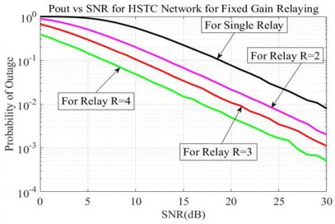
Figure 3. Outage probability for fixed gain relaying in HSTC Network
Figure 3 depicts the OP curves for fixed gain relaying with same settings as used previously. We can see that the analytical curves corresponding to computation from (31) agree well to the simulation results. Herein, the value of fixed gain C is computed using (32) for exact results. On comparing, one can see that the fixed gain relaying attains the same diversity order and has a comparable performance to that of variable gain relaying. However, the relative difference in performance can be attributed to their different coding gains, as reflected from the above example.
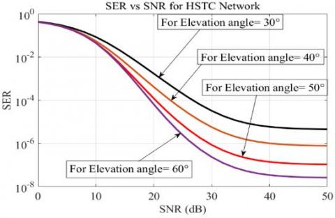
Figure 4. The effect of elevation angles of the satellite on symbol error rate (SER) in a situation where all connections are quasi-static i.e., ρ=1 and the different angel of elevation are equal i.e. $\phi_{S D}=\phi_{S R}=\phi_{R D}$.
Figure 4 depicts the effect of elevation angles of the satellite on the system's overall performance in a situation where all connections are quasi-static i.e., ρ=1 and different angle of elevations are equal i.e. $\phi_{S D}=\phi_{S R}=\phi_{R D}$. As may be observed in Figure 4, increasing elevation angles improves end-to-end performance significantly. It happens because high elevation angles produce good channel conditions with infrequent light shadowing (ILS) in satellite-terrestrial communications. As a result, the analytical values derived using the formula from (46) are similar to the simulation results, suggesting that the analytical framework established is accurate.
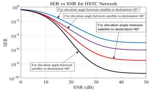
Figure 5. The effect of elevation angles of the satellite on symbol error rate (SER) in a situation where all connections are quasi-static faded i.e., $\rho=1$ and satellite to destination elevation angles $\phi_{S D} \in\left\{20^{\circ}, 40^{\circ}, 60^{\circ}, 80^{\circ}\right\}$ and $\phi_{S R}=\phi_{R D}=30^{\circ}$
Figure 5 depicts the effect of elevation angles of the satellite on the system's overall performance in a situation where all connections are quasi-static in nature i.e., ρ=1 and satellite to destination elevation angles $\phi_{S D} \in\left\{20^{\circ}, 40^{\circ}, 60^{\circ}, 80^{\circ}\right\}$ and $\phi_{S R}=\phi_{R D}=30^{\circ}$. The effectiveness of selective decode and forward-based collaboration in the Hybrid satellite-terrestrial cooperative (HSTC) network with time-selective satellite to destination links, relay to destination links, and satellite to relay links. In compared to the case where every connection undergoes quasi-static fading. i.e., ρ=1, it was discovered that time-selective fading caused by node mobility has a substantial impact on overall performance. As may be observed in Figure 5, increasing elevation angles improves end-to-end performance significantly. It happens because high elevation angles produce good channel conditions with infrequent light shadowing (ILS) in satellite-terrestrial communications. Furthermore, when relative speed increases, the degree of deterioration also increases, which may be illustrated by the diminishing channel correlation.
The performance evaluation for a selective DF cooperative hybrid satellite-terrestrial system with multiple relays is described and analyzed in this paper, where links in between satellite and the relay are assumed to be non-identical time-selective shadowed Rician faded and the link between relay and the destination terrestrial node is assumed to be non-identical time-selective over simplified Nakagami faded. Closed-form equations have been found for the per-frame average symbol error rate (SER) and the outage probability of HSTC systems. Simulation findings prove the influence of terrestrial node mobility and angle of elevation of the satellite on end-to-end performance (satellite and destination terrestrial node). The error rate of the HSTC is significantly low by increasing the elevation angle of the satellite on the relay point.
[1] Bu, Y.J., Lin, M., An, K., Ouyang, J., Yuan, C. (2016). Performance analysis of hybrid satellite–terrestrial cooperative systems with fixed gain relaying. Wireless Personal Communications, 89(2): 427-445. https://doi.org/10.1007/s11277-016-3278-9
[2] Bhatnagar, M.R., Arti, M.K. (2013). Performance analysis of AF based hybrid satellite-terrestrial cooperative network over generalized fading channels. IEEE Communications Letters, 17(10): 1912-1915. https://doi.org/10.1109/LCOMM.2013.090313.131079
[3] Bhatnagar, M.R., Arti, M.K. (2013). Performance analysis of hybrid satellite-terrestrial FSO cooperative system. IEEE Photonics Technology Letters, 25(22): 2197-2200. https://doi.org/10.1109/LPT.2013.2282836
[4] Varshney, N., Jagannatham, A.K. (2016). Capacity analysis for MIMO beamforming based cooperative systems over time-selective links with full SNR/one-bit feedback based path selection and imperfect CSI. In 2016 IEEE Wireless Communications and Networking Conference, pp. 1-6. https://doi.org/10.1109/WCNC.2016.7564776
[5] Sreng, S., Escrig, B., Boucheret, M.L. (2013). Exact symbol error probability of hybrid/integrated satellite-terrestrial cooperative network. IEEE Transactions on Wireless Communications, 12(3): 1310-1319. https://doi.org/10.1109/TWC.2013.013013.120899
[6] Shankar, R., Kumar, I., Mishra, R.K. (2019). Pairwise error probability analysis of dual hop relaying network over time selective Nakagami-m fading channel with imperfect CSI and node mobility. Traitement du Signal, 36(3): 281-295. https://doi.org/10.18280/ts.360312
[7] Varshney, N., Jagannatham, A.K. (2016). MIMO-STBC based multiple relay cooperative communication over time-selective Rayleigh fading links with imperfect channel estimates. IEEE Transactions on Vehicular Technology, 66(7): 6009-6025. https://doi.org/10.1109/TVT.2016.2634924
[8] Varshney, N., Krishna, A.V., Jagannatham, A.K. (2015). Selective DF protocol for MIMO STBC based single/multiple relay cooperative communication: End-to-end performance and optimal power allocation. IEEE Transactions on Communications, 63(7): 2458-2474. https://doi.org/10.1109/TCOMM.2015.2436912
[9] Xu, F., Lau, F.C., Yue, D.W. (2010). Diversity order for amplify-and-forward dual-hop systems with fixed-gain relay under Nakagami fading channels. IEEE Transactions on Wireless Communications, 9(1): 92-98. https://doi.org/10.1109/TWC.2010.01.090510
[10] Shankar, R., Kumar, I., Mishra, R.K. (2019). Outage probability analysis of MIMO-OSTBC relaying network over Nakagami-m fading channel conditions. Traitement du Signal, 36(1): 59-64. https://doi.org/10.18280/ts.360108
[11] Arti, M.K., Bhatnagar, M.R. (2014). Beamforming and combining in hybrid satellite-terrestrial cooperative systems. IEEE Communications Letters, 18(3): 483-486. https://doi.org/10.1109/LCOMM.2014.012214.132738
[12] Miridakis, N.I., Vergados, D.D., Michalas, A. (2014). Dual-hop communication over a satellite relay and shadowed Rician channels. IEEE Transactions on Vehicular Technology, 64(9): 4031-4040. https://doi.org/10.1109/TVT.2014.2361832
[13] An, K., Lin, M., Liang, T., Wang, J.B., Wang, J., Huang, Y., Swindlehurst, A.L. (2015). Performance analysis of multi-antenna hybrid satellite-terrestrial relay networks in the presence of interference. IEEE Transactions on Communications, 63(11): 4390-4404. https://doi.org/10.1109/TCOMM.2015.2474865
[14] An, K., Lin, M., Liang, T. (2015). On the performance of multiuser hybrid satellite-terrestrial relay networks with opportunistic scheduling. IEEE Communications Letters, 19(10): 1722-1725. https://doi.org/10.1109/LCOMM.2015.2466535
[15] Shankar, R., Kumar, I., Kumari, A., Pandey, K.N., Mishra, R.K. (2017). Pairwise error probability analysis and optimal power allocation for selective decode-forward protocol over Nakagami-m fading channels. In 2017 International Conference on Algorithms, Methodology, Models and Applications in Emerging Technologies (ICAMMAET), pp. 1-6. https://doi.org/10.1109/ICAMMAET.2017.8186700
[16] Gradshteyn, I.S., Ryzhik, I.M., Romer, R.H. (1988). Tables of integrals, series, and products. 6th ed. New York, NY, USA: Academic, 56(10): 958. https://doi.org/10.1119/1.15756
[17] Khattabi, Y., Matalgah, M.M. (2014). Performance analysis of AF cooperative networks with time-varying links: Error rate and capacity. In 2014 Wireless Telecommunications Symposium, pp. 1-6. https://doi.org/10.1109/WTS.2014.6835001
[18] Wang, H.S., Chang, P.C. (1996). On verifying the first-order Markovian assumption for a Rayleigh fading channel model. IEEE Transactions on Vehicular Technology 45(2): 353-357. https://doi.org/10.1109/25.492909
[19] Kumar, I., Kumar, A., Kumar Mishra, R. (2022). Performance analysis of cooperative NOMA system for defense application with relay selection in a hostile environment. The Journal of Defense Modeling and Simulation. https://doi.org/10.1177/15485129221079721
[20] Sachan, V., Kumar, I., Bhardwaj, L., Mishra, R.K. (2020). Pairwise error probability analysis of SM-MIMO system employing k–μ fading channel. Procedia Computer Science, 167: 2516-2523. https://doi.org/10.1016/j.procs.2020.03.304
[21] McKay, M.R., Zanella, A., Collings, I.B., Chiani, M. (2009). Error probability and SINR analysis of optimum combining in Rician fading. IEEE Transactions on Communications, 57(3): 676-687. https://doi.org/10.1109/TCOMM.2009.03.060521
[22] Kumar, I., Sachan, V., Shankar, R., Mishra, R.K. (2018). An investigation of wireless S-DF hybrid satellite terrestrial relaying network over time selective fading channel. Traitement du Signal, 35(2): 103-120. https://doi.org/ 10.3166/ts.35.103-120
[23] Kumar, I., Mishra, R.K. (2020). Performance analysis for wireless non-orthogonal multiple access downlink systems. In 2020 International Conference on Emerging Frontiers in Electrical and Electronic Technologies (ICEFEET), pp. 1-6. https://doi.org/10.1109/ICEFEET49149.2020.9186987
[24] Iqbal, A., Ahmed, K.M. (2011). A hybrid satellite-terrestrial cooperative network over non identically distributed fading channels. J. Commun., 6(7): 581-589.
[25] Lin, M., Ouyang, J., Zhu, W.P. (2014). On the performance of hybrid satellite-terrestrial cooperative networks with interferences. In 2014 48th Asilomar Conference on Signals, Systems and Computers, pp. 1796-1800. https://doi.org/10.1109/ACSSC.2014.7094777
[26] An, K., Lin, M., Ouyang, J., Huang, Y., Zheng, G. (2014). Symbol error analysis of hybrid satellite–terrestrial cooperative networks with cochannel interference. IEEE Communications Letters, 18(11): 1947-1950. https://doi.org/10.1109/LCOMM.2014.2361517
[27] Kumar, I., Mishra, R.K. (2020). An efficient ICI mitigation technique for MIMO-OFDM system in time-varying channels. Mathematical Modelling and Engineering Problems, 7(1): 79-86. https://doi.org/10.18280/mmep.070110
[28] Kumar, I., Sachan, V., Shankar, R., Mishra, R.K. (2020). Performance analysis of multi-user massive MIMO systems with perfect and imperfect CSI. Procedia Computer Science, 167: 1452-1461. https://doi.org/10.1016/j.procs.2020.03.356
[29] Bhatnagar, M.R. (2014). Performance evaluation of decode-and-forward satellite relaying. IEEE Transactions on Vehicular Technology, 64(10): 4827-4833. https://doi.org/10.1109/TVT.2014.2373389
[30] Arti, M.K., Bhatnagar, M.R. (2014). Two-way mobile satellite relaying: A beamforming and combining based approach. IEEE Communications Letters, 18(7): 1187-1190. https://doi.org/10.1109/LCOMM.2014.2323307