Anupama K Channappa* | Nagaraja Ramaiah | Shivakumar B Rajanna
© 2022 IIETA. This article is published by IIETA and is licensed under the CC BY 4.0 license (http://creativecommons.org/licenses/by/4.0/).
OPEN ACCESS
In the cloud environment, the process of task scheduling and resource allocation plays a vital role in cloud resource management. The unpredictable and uncertain behaviour of the task arrival rate poses significant challenges in the effective allocation of resources. An efficient scheduling technique is essential to avoid under or overutilization of resources. In order to increase the performance of scheduling and allocation, this paper presents multi-objective optimization method for optimal resource allocation and task scheduling based on a three-stage strategy. In the first stage, a description of tasks and virtual machines is prepared. At stage two, tasks are classified and labelled based on the resource demand and execution time. Finally, the modified-Grey Wolf optimization algorithm is used for the allocation and scheduling of tasks for a disparate scenario. The experimental results proved that the proposed method reduced the makespan time and cost with an improved utilization rate.
cloud computing, scheduling, resource allocation, multi-objective optimization, modified-grey wolf optimization algorithm
Cloud computing has become very popular in the area of leasing or renting cloud resources. The pay-as-you-go model of the cloud attracts the organizations and individual users to execute their applications on the cloud. Applications may vary in size, resource requirement (compute/memory/storage) and execution time (long/short). These applications at the cloud end are divided into separate executables called as jobs, tasks and instances. Based on the attributes of the task, the cloud service providers (CSP) must be capable of handling the varied requests of their clients by creating virtual machines (VM) in cloud. The main aim of the CSP is to minimize, the cost, Service Level Agreements (SLA) violations, while maximizing resource utilization and ultimately maintaining good Quality of Service (QoS) [1].
Cloud users submit their application through internet portal and these applications in-turn divided as tasks. Every task has its own characteristics and must complete its execution in a given stipulated amount of time. The variable and uncertain behaviour of task arrival rate hinders service providers to execute the task in the given time which leads to performance degradation and the purpose of the cloud usage is not met. This situation creates significant issue to the service providers and it is essential to provide a feasible solution to improve performance and QoS of the cloud system. The skilful solution to overcome task failure is the need for implementing a challenging scheduling and allocation strategies. Various scheduling policies have been implemented to overcome task failures and made an attempt to minimize the execution time, energy consumption, cost, SLA violation rate etc. [2-4]. Many researchers proposed multi-objective task scheduling using nature inspired algorithms and few developed novel approaches for task scheduling and optimal resource allocation [5]. Another efficient way of task scheduling is achieved by classifying the tasks based on historical data and similarly creating different types of VM’s so as to cater the task demand.
Major shortfalls found during scheduling and allocation are the assignment of the tasks to VM’s. Suppose if larger tasks are allocated to the VM’s having less processing capability will apparently consume long processing time to complete its execution and at times not before the tasks’ deadline. In the same scenario, short-range tasks have to wait until the completion of the previously allocated task, thereby reducing the overall performance of the clouds. One such solution to overcome such imbalance is to create and group VM’s of various sizes and assign the tasks to the appropriate VM’s with appropriate resources [6, 7]. By doing so, the virtual machine creation and task waiting time can be reduced eventually avoiding task failures.
To overcome the existing shortcomings, we propose three-stage strategy for task scheduling and resource allocation model using Modified Grey Wolf algorithm (mGWO). The main objective of the proposed method is to minimize makespan and cost while maximizing utilization of cloud resources. The entire work is divided into three stages. In the first stage, the model determines the characteristics of the task and the VM’s. In the second stage, the tasks are labelled based on the historical task data and also on the observations made in earlier research works using real world datasets [8-10]. These tasks are classified and grouped as small, large, compute and memory intensive tasks. Each group of tasks are stored and maintained as a separate queue. Likewise, corresponding VM’s are created beforehand that are most suitable for handling task scheduling. In the final stage, nature inspired algorithm is applied for task scheduling and resource allocation. The proposed task scheduling algorithm uses modified grey wolf optimization algorithm to minimize makespan, cost and to improve cloud resource utilization.
The key contribution of the proposed work is summarized as follows.
The proposed model classifies the tasks based on their characteristics and similarly VM’s, which aids in assigning tasks to the most suitable VM’s.
An efficient optimal resource allocation and management method is proposed using a modified grey wolf optimization algorithm.
The performance of the proposed model is tested against other existing algorithms considering different scenarios by varying tasks numbers.
The rest of the paper is organized as follows: Related works on task scheduling in the cloud are given in section 2; Problem formulation and mathematical models are explained in section 3; Section 4 focusses on the methodology; The experimental setup, results and analysis are discussed in Section 5; Finally, the work is summarized with future scope.
The review of related works in the field of resource allocation and task scheduling in the cloud is discussed in this section. With recent developments, task scheduling in cloud computing has emerged as a multi-objective optimization problem with different optimization goals.
Pang et al. [11] proposed a hybrid algorithm for scheduling based on estimation of distribution and genetic algorithm (EDA-GA). The algorithm has attained fast convergence speed and strong searching ability. The proposed work mainly focused on load balancing and task completion time. The experimental results effectively reduced the completion time and improve the load balancing ability. Li et al. [12] solve task scheduling problems using a hybrid discrete artificial bee colony algorithm (ABC). Here both single and multi-objective are considered. To enhance searching capabilities an improved perturbation structure is embedded in the proposed algorithm. An efficient selection and update method is used for further improvement in exploration and exploitation ability. The work mainly focuses on minimizing the makespan and minimizing the device and total workloads of all the devices. The results proved to be efficient and more robust when tested on different scale problems along with different problem structures.
Sanaj and Pratap [13] developed a chaotic squirrel search algorithm (CSSA) for scheduling tasks in IaaS cloud environment. Authors have considered energy, cost, task completion time, resource utilization and SLA violation as performance metrics for evaluation. The findings demonstrate that the proposed model can identify a better cost-effective solution when compared with other existing methods.
Jacob et al. [14] suggested a hybrid task scheduling approach by combining cuckoo search and particle swarm optimization (CPSO) to optimize and improve the scheduling performance and costs. The main advantage of the CPSO algorithm is its quick convergence thus making the scheduling approach to get a near-optimal solution. The algorithm aims to reduce makespan, deadline violation rate and all cost factors which include user and performance cost.
The literature review extends to focus on different variants of the grey wolf optimization algorithm for solving multi-objective task scheduling problems. For reducing issues related to scheduling, Natesan and Chokkalingam [15] have proposed a modified mean grey wolf optimization algorithm which mainly focuses on minimizing execution time and energy consumption. Both encircling and hunting equations are modified in this method. Hence the modified algorithm aids in maximizing the efficiency of the motion and finding a suitable path for the wolf in the search area. The experiment has been conducted on both normal and uniform datasets workloads. The obtained results prove that the proposed algorithm achieves improvement in makespan and energy consumption when compared with standard GWO and other existing algorithms. Natesan and Chokkalingam [16] also proposed an improved GWO algorithm called performance-cost grey wolf optimization algorithm (PCGWO) to achieve optimization in the scheduling and allocation process in cloud computing. The main aim of the algorithm is to minimize the processing time and cost so that the maximum number of tasks are executed within the task deadline. The performance analysis results show an excellent reduction in the time and cost when compared with traditional algorithms but the results are not compared with other existing meta-heuristic methods.
Sheetal and Ravindranath [17] established a model for allocating resources in the cloud using the democratic grey wolf optimization (DGWO) algorithm. The benefit of using DGWO is its high-speed convergence, easy implementation and improved searching optimum time. The performance of the proposed work is evaluated using parameters like makespan, energy consumption and time-based evaluation. The research proved to achieve better results in terms of turnaround time, throughput and time-based evaluation when compared with HABCSS, krill herd and SFLA-CS.
The improved chaotic binary grey wolf optimization [IGWO] algorithm proposed by Mohammadzadeh et al. [18] focuses on increasing the convergence speed of the algorithm and preventing falling into local optimum. The Chaos theory and hill-climbing methods are used by the improved GWO algorithm. The binary version of the proposed algorithm deals with workflow scheduling algorithm using various S function and V functions. In this paper, the authors aimed to minimize the execution cost, power and makespan of the system. The experiment was conducted on scientific workflows of various sizes and the proposed method proved to achieve better results when compared with other metaheuristic algorithms.
To solve multi-objective task scheduling problems in the cloud environment Sreenu and Malempati [19] proposed Fractional Greywolf Multi-objective optimization-based Task Scheduling strategy (FGMTS) an enhanced grey wolf optimization algorithm by integrating the existing fractional theory. The resources are allocated to tasks, considering QoS constraints through minimizing execution time, communication time, energy consumption and better resource utilization. The experiment was performed over two cloud setups by varying the number of physical machines, virtual machines and tasks. Sreenu and Malempati [20] also proposed xMFGMTS algorithm, a modified variety of FGMTS. The proposed method uses an epsilon-constraint and penalty-cost function for computing execution time, communication time, execution cost, communication cost, resource utilization and energy. The algorithm uses an additional term to update the position in combination with alpha and beta solutions in order to select better solutions. The performance of the proposed methods was evaluated over existing scheduling methods: PSO, GWO and GA. The results proved to be effective and produced a stable and acceptable solution in the process of task scheduling.
The authors [21-23] have developed a scheduling approach based on task classification. In the proposed methods, tasks are classified according to the resource demand. Similar types of tasks are merged and scheduled to minimize task execution cost, energy and maximize resource utilization. Task classification aids in the creation of the actual number and type of virtual machines required for allocating the resource. Overall observation summarizes that better performance can be obtained by jointly combining optimization using metaheuristic techniques during the process of task allocation and scheduling.
This section provides the description of makespan, cost and utilization which are considered as multi-objective functions for optimal task scheduling in the proposed work. The fitness value is calculated using Eq. (1), Eq. (6) and Eq. (8). The mathematical notations, symbols used in this paper and corresponding explanations are listed in Table 1.
Table 1. Notations and explanations
|
$\mathrm{T}=\left\{T_{1}, T_{2}, T_{3}, \ldots \ldots T_{n}\right\}$ |
Set of Tasks |
|
$\mathrm{V}=\left\{V_{1}, V_{2}, V_{3} \ldots \ldots . V_{m}\right\}$ |
Set of Virtual machines |
|
$T_{i}$ |
jth Task |
|
$V_{i}$ |
ith Virtual machine |
|
$T_{j i}$ |
Task j on virtual machine i |
|
$\boldsymbol{C}_{i}, \boldsymbol{M}_{\boldsymbol{i}}$ |
CPU and memory of virtual machine Vi |
|
$\boldsymbol{C}_{\boldsymbol{j}}, \boldsymbol{M}_{\boldsymbol{j}}, \boldsymbol{E}_{\boldsymbol{j}}$ |
CPU, memory and Execution time of task Tj |
|
$D_{j}$ |
Deadline of task Tj |
|
$\boldsymbol{S}_{j}$ |
Start time of task Tj |
|
$W_{j}$ |
Weight of the task Tj |
|
$Q_{V S}, Q_{V C}, Q_{V M}, Q_{V L}$ |
Queues of S, CI, MI and L VM |
|
$Q_{T S}, Q_{T C}, Q_{T M}, Q_{T L}$ |
Queues of S, CI, MI and L tasks |
|
$T_{j}^{s}, T_{j}^{c}, T_{j}^{m}, T_{j}^{l}$ |
Task Tj in the queue after classification as S, CI, MI and L tasks |
A Multi-objective optimization: To solve the problem of task scheduling and allocation, the work considers more than one objective. The three important objectives which are considered in the proposed work are the makespan, cost and utilization. When solving multi-objective problems, multiple optimal solutions are available for the problem and need to choose one among them.
General multi-objective optimization problem is given as follows:
f(x) = [f1(x), f2(x)…..fm(x)]
x = [x1,x2,x3…….xn]
‘m’ denotes the number of objectives, for any multi-objective optimization, $\mathrm{m} \geq 2$, in this case m=3.
The feasible solutions are indicated by x1, x2, x3… xn, such that $X \in x$, where X is a feasible solution set.
3.1 Makespan
Assuming that every task is allocated to a single VM and the tasks are not pre-empted during the execution, makespan is the maximum time taken by the virtual machine to complete the execution of all tasks as in Eq. (1).
$\operatorname{Makespan}(x)=\max \sum_{j=1}^{n} C T_{i j}$ (1)
where, $C T_{i j}$ implies the total completion time of set of $j$ th tasks on $i^{\text {th }}$ virtual machine and $\mathrm{n}$ is the total number of tasks [24].
3.2 Cost model
Every task submitted by the user is different in nature, some of the tasks may either require more memory or more CPU. In addition, there is a difference in the costs for resources. Thus, based on the resource requirement, task costs also vary. The work considers minimizing the cost function. The total resource cost is calculated by adding the CPU and memory cost function of the virtual machine [25, 26]. The cost functions of CPU and memory of virtual machine are calculated as in Eq. (2) and Eq. (3).
$C(x)=\sum_{i=1}^{m} C_{c o s t}(i)$ (2)
$M(x)=\sum_{i=1}^{m} M_{\text {cost }}(i)$ (3)
where, $C_{\text {cost }}(i)$ and $M_{\text {cost }}(i)$ are the cost of CPU and memory of $i$ th virtual machine $\left(V_{i}\right)$.
The following Eq. (4) is used to calculate the cost associated to CPU:
$C_{\text {cost }}(i)=C_{b} \times C_{i} \times t_{i j}+C_{t}$ (4)
where, $C_{b}$ represents the base cost, $C_{i}$ is the CPU of virtual machine $V_{i}, t_{i j}$ denotes the run time duration of task $t_{j}$. The transmission cost of CPU is given by $C_{t}$. Here $C_{b}$ and $C_{t}$ are constants where Cbase $=0.17 / \mathrm{hr}$ and CTrans $=0.005[25]$. Similarly, the memory cost is defined using Eq. (5).
$M_{\operatorname{cost}}(i)=M_{b} \times M_{i} \times t_{i j}+M_{t}$ (5)
Here, the base cost of memory is given by $M_{b}, M_{i}$ indicates the memory of the virtual machine $V_{i} \cdot t_{i j}$ signifies the processing time of $j^{t h}$ task on $i^{t h}$ virtual machine and $M_{t}$ represents the transmission cost of memory. The values of $M_{b}$ and $M_{t}$ are fixed where $M_{b}=0.05 / \mathrm{GB} /$ hour and $M_{t}=0.50[25]$. The overall cost function $\operatorname{Cost}(\mathrm{x})$ is calculated as in Eq. (6) using Eq. (2) and Eq. (3).
$\operatorname{Cost}(x)=C(x)+M(x)$ (6)
3.3 Utilization
In cloud systems, every resource is valued with a certain cost as perceived from the above cost model. Therefore to minimize the cost an efficient utilization of the total available resource is essential [27]. The utilization of a virtual machine is the fraction of the overall makespan and calculated as in Eq. (7).
$U[v m]=\frac{\text { Makespan }[v m]}{\text { Makespan }}, 1 \leq v m \leq m$ (7)
The utilization value of the VM is placed between 0 and 1. The average VM utilization $U_{A v g}$ is the proportion of summation of all makespan and the value of total VM’s multiplied with makespan and is calculated using Eq. (8).
$U_{A v g}=\frac{1}{\text { Makespan } * m} \sum_{i=1}^{m}$ Makespan $[m]$ (8)
The average utilization values are found in the range 0 to 1. If the value of $U_{A v g}=1$ indicates fully loaded VM’s.
3.4 Fitness function calculation
Every search agent in the population produces a feasible solution. The quality of the obtained solutions are evaluated using the fitness function. Since this work intends to minimize makespan, cost and maximize utilization the fitness function is defined as in Eq. (9).
$F=\left[\varphi_{1}(\right.$ Makespan $)+\varphi_{2}($ Cost $)+\varphi_{3}($ Utilization $\left.)\right]\varphi_{1}+\varphi_{2}+\varphi_{3}=1 ;\left(0 \leq \varphi_{1}, \varphi_{2}, \varphi_{3} \leq 1\right)$ (9)
Here $\varphi_{1}, \varphi_{2}$ and $\varphi_{3}$ denotes weight coefficients of makespan, cost and utilization. The values are set to 0.5, 0.3 and 0.2 which means the first objective makespan is given the highest importance than cost and utilization [12].
Figure 1. Task scheduling and resource allocation model
This section describes the proposed resource allocation and task scheduling model for the cloud data center. In the cloud environment, the applications are submitted by the users to the cloud service providers for its execution. These applications are further divided into tasks or jobs. Every task is heterogeneous in nature in terms of resource demand, execution time, deadline and task length. In the task queue, all the incoming tasks are pooled and wait for their turn to execute. Based on the resource requirement and execution time, the tasks are classified and sent to the task buffer queue. Here four queues are formed for four different types of tasks such as small(S), compute-intensive (CI), memory-intensive (MI), and large (L). Here classified tasks are maintained as separate queues and are sorted in ascending order based on the weight value calculated using deadline and execution time. At the other end, four types of VM’s are created and the resource manager (RM) provides information about the available virtual machines with their CPU and memory capacity. Based on the resource availability, the list of VM’s is also sorted and maintained as separate queues in the task-resource avail list table. The scheduler checks the task-resource avail list table and based on the task’s resource requirement an optimal allocation strategy is applied to select appropriate VM’s and tasks are scheduled accordingly. After the successful execution of the task, the resources are released and the task-resource avail list table is updated. The entire working principles of the proposed system is depicted in Figure 1 in three stages. The following sections describe each stage in detail.
4.1 Stage 1: Description of task and virtual machines
Let us assume that there are $\mathrm{N}$ finite set of incoming tasks, $\mathrm{T}=\left\{T_{1}, T_{2}, T_{3}, \ldots \ldots T_{n}\right\}$ submitted by different users with specific resource demand. Let attributes of Task $T_{j}=\left(\boldsymbol{C}_{\boldsymbol{j}}, M_{j}\right.$, $\left.L_{j}, S_{j}, E_{j}, D_{j}\right)$. The symbol $C_{j}$ denotes CPU usage, $M_{j}$ represents memory requirement, $L_{j}$ signifies the task length, $S_{j}, E_{j}$ and $D_{j}$ indicates the start time, execution time and deadline of the task $T_{j}$ respectively. Based on the application, the task requests for different type of resources for its successful execution. Characteristics of the Virtual machines are described as follows:
Let there exists $M$ number of virtual machines, $\mathbf{V}=\left\{V_{1}, V_{2}\right.$, $\left.V_{3} \ldots \ldots . V_{m}\right\}$, hosted by physical machines residing in the datacenter. Each VM in the cloud are defined with a set of parameters.
Let $V_{i}=\left(C_{i}, M_{i}, B_{i}, S_{i}\right)$ representing $\mathrm{CPU}$, memory, bandwidth and storage of the $V_{i}^{\text {th }} \mathrm{VM}$ respectively.
4.2 Stage 2: Task labelling and classification
Cloud users submit the tasks which demands variety of resources for its successful execution. Some tasks demand for more CPU than memory and few tasks may require large amount of memory and some case tasks may demand for both the resource but varying with the execution time. Considering the task’s characteristics task classifier categorizes tasks as process intensive, memory intensive, short and long running tasks [21-23].
In this work criteria for classification of tasks considers both the resource demand and execution time of the task. By examining the characteristics of the incoming tasks, the tasks are classified and buffered into separate queue. The classification of the tasks is performed as mentioned in Figure 2. For instance, if any task requests for more CPU cores, then the classifier directs such tasks to reside in compute-intensive queue. In reality, it is found that majority of the tasks are found to have short execution duration [28]. Finally, the list of classified tasks are sorted and maintained in the task-resource avail list table for further task scheduling purpose.
4.2.1 Task Queue
Assuming that CPU-avg is the average CPU requirement of any task for successful execution, mem-avg is the average memory used by any task and ET-avg is the average task execution time, task is classified as in the Figure 2. As per the algorithm, let us consider that there are K set of tasks, where K = {w, x, y, z} that are classified into four different queues namely: $Q_{T S}, Q_{T C}, Q_{T M}, Q_{T L}$ of small, compute-intensive, memory-intensive and large tasks respectively.
$Q_{T S}=\left\{T_{1}^{S}, T_{2}^{S} \ldots \ldots \ldots T_{j}^{S} \ldots T_{w}^{s}\right\}$
$Q_{T C}=\left\{T_{1}^{c}, T_{2}^{c} \ldots \ldots \ldots T_{j}^{c} \ldots T_{x}^{c}\right\}$
$Q_{T M}=\left\{T_{1}^{m}, T_{2}^{m} \ldots \ldots \ldots . T_{j}^{m} \ldots T_{y}^{m}\right\}$
Q $_{T L}=\left\{T_{1}^{l}, T_{2}^{l} \ldots \ldots \ldots T_{j}^{l} \ldots T_{z}^{l}\right\}$
For instance, if task’s CPU usage $C_{j} \geq T^{C P U_{-} a v g}$ then, that task is sent to QTC queue and the task is referred as $T_{j}^{c}$.Similarly, as per the classification algorithm, all the tasks are classified and stored as separate queues. The total number of tasks at any instant is the sum of all the tasks in each queue.
4.2.2 Virtual machine queue
In the cloud, achieving maximum resource utilization and maintaining good QoS can be achieved through an efficient resource allocation method. The resource manager in the cloud maintains the list of available resources which are ready to use for allocating the task. The knowledge about the task description helps in creating VM’s of different types and sizes meeting the requirements of the task. Based on the size of the VM, the resource manager sorts all the available VM’s and forms four queues of VMs as follows:
$\begin{aligned} \mathrm{Q}_{\mathrm{vs}} &=\left\{V_{1}^{s}, V_{2}^{s}, \ldots V_{i}^{s} \ldots \ldots V_{n}^{s}\right\} \\ \mathrm{Q}_{\mathrm{VC}} &=\left\{V_{1}^{c}, V_{2}^{c}, \ldots V_{i}^{c} \ldots \ldots V_{n}^{c}\right\} \\ \mathrm{Q}_{\mathrm{VM}} &=\left\{V_{1}^{m}, V_{2}^{m}, \ldots V_{i}^{m} \ldots . V_{n}^{m}\right\} \\ \mathrm{Q}_{\mathrm{VL}} &=\left\{V_{1}^{l}, V_{2}^{l}, \ldots V_{i}^{l} \ldots \ldots \ldots V_{n}^{l}\right\} \end{aligned}$
The VM queues QVS, QVC, QVM and QVL represents small, compute-intensive, memory-intensive and large tasks executable capacity VMs respectively. The VM categorization formed on the CPU speed and RAM size is provided in Table 2 of section 5.
4.2.3 Task-Resource Avail List Table
Classified tasks from each queue is then mapped to the respective queue maintained in the task-resource avail list table. In each queue, for every task $T_{j}$, weight $W_{j}$ is calculated as in Eq. (10):
$W_{j}=\frac{D_{j}-S_{j}}{E_{j}}$ (10)
where, $D_{j}$ - Deadline of task, $S_{j}$ - Start time of task $\mathrm{T}_{\mathrm{j}}, E_{j}-$Execution time of task Tj .
Using Eq. (10), the weights of all the tasks in the particular queue are calculated. The value of the weight helps in scheduling the earliest deadline first task. For example, if the weights of the tasks are 1,2,3…etc., then the task having lowest value will be queued first for the execution. Each queue is sorted based on the weights and are ready for mapping to the appropriate VM’s for execution. The task-resource avail list table also maintains the list of available virtual machines received from resource manager. The scheduler fetches the information of both waiting task and the list of available appropriate VM’s for allocating tasks to VM’s. After the allocation and execution process of task $T_{j}$ on virtual machine $V_{i}$, the allocated resources are released and added to the virtual resource pool. Understanding the characteristics of the tasks helps in better virtual resource management. For example, assigning a long running task to a VM having large CPU and Memory capacity and short running tasks to VM with lower processing capability, thus improving makespan and overall throughput of the system.
4.3 Stage 3: Task scheduling and resource allocation
The main aim of the proposed multi-objective scheduling problem is to assign the task to VM of the proper size to minimize makespan, cost and resource utilization. As understood from the previous sections the user’s task demands a certain amount of resources and timely allocation of the requested resources is a challenging task in scheduling. Assuming that there are n individual tasks of different types and are assigned to the appropriate size VM’s while attaining multiple objectives. The process of task classification and resource allocation algorithm is depicted in Figure 2. Flow diagram of the task scheduling and resource allocation is represented in Figure 3.
Figure 2. Proposed task scheduling and resource allocation algorithm
Figure 3. Flow diagram of task scheduling and resource allocation
4.4 Overview of modified grey wolf optimizer algorithm (mGWO)
This section describes the mathematical model of social hierarchy, encircling prey, hunting and attacking prey are provided. End of this section outlines pseudocode of the algorithm [29, 30].
4.4.1 Social hierarchy and searching for the prey (exploration)
Typical Grey Wolf Optimizer (GWO) mimics the social hierarchy and hunting mechanism of grey wolves in nature. The dominating or the fittest solution is considered as alpha (α). Apart from α, the second and third best fit solution are called beta (β) and delta ($\delta$). The remaining lowest ranking solutions are assumed as omega (ω) in the hierarchy. The GWO algorithm contemplates only α, β and δ for optimization purpose. Wolves wander in search of the location of the prey. They disperse away during the searching of the prey and gather while attacking the prey.
4.4.2 Encircling prey
During the process of hunting grey wolves encircle the prey. Following equations gives the mathematical model of the encircling behavior is as in Eq. (11) and Eq. (12):
$\vec{X}(t+1)=\overrightarrow{X_{p}}(t)-\vec{A} \cdot \vec{D}$ (11)
$\vec{D}=\left|\vec{C} \cdot \overrightarrow{X_{p}}(t)-\vec{X}(t)\right|$ (12)
where, $\vec{X}(t)$ and $\vec{X}(t+1)$ are the current and the next location of the wolf. $\vec{A}$ and $\vec{C}$ are the coefficient vectors, $\mathrm{t}$ indicates the current iteration, $\overrightarrow{X_{p}}$ and $\vec{X}$ corresponds the position vector of the prey and the grey wolf. The values of vector $\vec{D}$ depends on the position $\overrightarrow{X_{p}}$ of the prey. The coefficient vectors $\vec{A}$ and $\vec{C}$ are calculated as in Eq. (13) and Eq. (14):
$\vec{A}=2 \vec{a} \cdot \overrightarrow{r_{1}}-\vec{a}$ (13)
$\vec{C}=2 \cdot \overrightarrow{r_{2}}$ (14)
where, $r_{1}$ and $r_{2}$ are random vectors in the interval $[0,1]$ and the component of vector $\vec{a}$ values are linearly decreased from 2 to 0 over the course of iterations.
4.4.3 Hunting
Grey wolves have the capability to identify the location of the prey. Habitually the alpha guides the hunt. The beta and delta will participate occasionally. Thus alpha, beta and delta will have better knowledge about the prospective location of the prey. The objective of the algorithm is to find minimum in the search landscape. The algorithm assumes that the positions of alpha as the best candidate solution, beta and delta as the next best solutions in the entire population. The remaining solutions like omega update their positions according to these three best positions. This hunting behavior is modelled as in Eq. (15), Eq. (16) and Eq. (17):
$\overrightarrow{D_{\alpha}}=\left|\overrightarrow{C_{1}} \cdot \overrightarrow{X_{\alpha}}-\vec{X}\right|, \overrightarrow{D_{\beta}}=\left|\overrightarrow{C_{2}} \cdot \overrightarrow{X_{\beta}}-\vec{X}\right|, \overrightarrow{D_{\delta}}=\left|\overrightarrow{C_{3}} \cdot \overrightarrow{X_{\delta}}-\vec{X}\right|$ (15)
$\overrightarrow{X_{1}}=\overrightarrow{X_{\alpha}}-\overrightarrow{A_{1}} \cdot\left(\overrightarrow{D_{\alpha}}\right), \overrightarrow{X_{2}}=\overrightarrow{X_{\beta}}-\overrightarrow{A_{2}} \cdot\left(\overrightarrow{D_{\beta}}\right), \overrightarrow{X_{3}}=\overrightarrow{X_{\delta}}-\overrightarrow{A_{3}} \cdot\left(\overrightarrow{D_{\delta}}\right)$ (16)
$\vec{X}(t+1)=\frac{\overrightarrow{X_{1}}+\overrightarrow{X_{2}}+\overrightarrow{X_{3}}}{3}$ (17)
4.4.4 Attacking the prey (exploitation)
Grey wolves complete its hunting process by attacking the prey. The mathematical model for attacking the prey is by decreasing the value of $\vec{a}$ in various iterations. The value of the parameter $\vec{A}$ is based on $\vec{a}$, which linearly reduces from 2 to 0 . Due to randomness, the values of $\vec{A}$ are placed in the interval [-2a, 2a].
When the values of $\vec{A}$ are: $1<\vec{A}<-1$ promotes exploration, whereas exploitation is emphasized when $-1<\vec{A}<1$.
To find an accurate global optimum there is a need of good balance between exploration and exploitation. It is found that higher the exploration results greater randomness. In addition, too much exploitation results too little randomness. Balance between exploitation and exploration is achieved by updating mechanism. As emphasized above, GWO algorithm devotes half of the iterations to exploration and the remaining half of the iterations for exploitation. But mGWO employs exponential function to reduce the value of $\vec{a}$ during the course of iterations using the update Eq. (18).
$a=2\left(1-\frac{t^{2}}{T^{2}}\right)$ (18)
where, t indicates the current iteration and T specifies the maximum number of iterations. In mGWO 70% of the iterations are used for exploration and 30% of the iterations for exploitation. The pseudocode for the mGWO algorithm is given in Figure 4.
Figure 4. Pseudo code of mGWO algorithm
5.1 Experimental details
The performance of the proposed system was evaluated using the CloudSim toolkit simulator [31]. The experiments are conducted on windows10 with an 8GB memory machine. For the experiment, four types of VM’s and four types of tasks are considered. The number of VM’s are fixed to 20 of each type and the task length is randomly generated within the specified range as shown in Table 2. The task parameter settings are shown in Table 3. The experiment is evaluated by varying the number of tasks from 100 to 500 and compared with existing algorithms: PSO, CSO and GWO [15, 19, 20]. To simulate as that of real cloud computing, the experiment is conducted by considering two scenarios:
Scenario-1: Few large quantities of $T_{j}^{S}$ tasks with relatively less quantity of $T_{j}^{c}, T_{j}^{m}, T_{j}^{l}$ tasks.
Scenario-2: $T_{j}^{S}, T_{j}^{c}, T_{j}^{m}$ and $T_{j}^{l}$ tasks are randomly determined.
Table 2. Virtual machines with speed & memory
|
VM Type |
Type 1 Small |
Type 2 MI |
Type 3 CI |
Type 4 Large |
|
MIPS |
1000 |
2000 |
8000 |
8000 |
|
RAM (GB) |
1 |
8 |
2 |
8 |
Table 3. Parameter settings of tasks
|
Task Type |
S |
MI |
CI |
L |
|
Length (MI) |
100-1000 |
1000-4000 |
8000-10000 |
4000-10000 |
The simulator uses random number generator for generating tasks of different types in the specified range. In scenario-1, $70 \%$ of the tasks were of $T_{j}^{S}$ type, and $10 \%$ each of $T_{j}^{c}, T_{j}^{m}, T_{j}^{l}$ type tasks are considered. In Scenario-2, the quantity of each task type $T_{j}^{S}, T_{j}^{c}, T_{j}^{m}$ and $T_{j}^{l}$ are not fixed but are randomly chosen. To simulate the proposed method, few assumptions are made as follows:
Tasks are independent and each task is allocated to one VM, tasks and VM’s are heterogeneous in nature.
Assuming that every task is allocated to a single VM and the tasks are not pre-empted during the execution.
Task resource requirement is always less than the available resource.
5.2 Performance of the proposed model
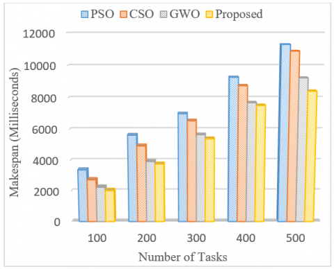
This section evaluates and compares the simulation results obtained for the metrics like makespan, cost and resource utilization. The tasks are executed in the order of 100 to 500 in both scenarios. The main goal of the proposed work is to minimize the task execution time and cost while maximizing resource utilization. The x-axis represents the makespan in milliseconds and the y-axis the number of tasks. It is observed that both the proposed and GWO schedules the tasks efficiently when compared with PSO and CSO algorithms.
The overall makespan values obtained after scenario-1 and scenario-2 are depicted in Figure 5 and Figure 6 respectively.
Figure 5. Makespan value comparisons for Scenario-1
Figure 6. Makespan value comparisons for Scenario-2
As observed in scenario-2, the obtained makespan values are not linear due to the random pattern of task arrival with varied task lengths.
As the number of tasks increases the makespan time calculated by the proposed method is always lower than the other three algorithms. The rate of improvement in the performance of the proposed work when compared with PSO, CSO and GWO for scenario-1 show 39.72%,25.59% and 9.74% improvements in makespan time whereas, 44.34%, 37.52% and 6.56% for scenario-2.
Figure 7. Cost value comparisons for Scenario-1
Figure 8. Cost value comparisons for Scenario-2
Figure 9. Resource Utilization for Scenario-1
Figure 10. Resource Utilization for Scenario-2
Table 4. Utilization of vm’s in scenario-1 and scenario-2
|
Resource Utilization by different type of VM’s in Scenario-1 |
|||||
|
VM Type / No. of Tasks |
100 |
200 |
300 |
400 |
500 |
|
Small |
0.68396 |
0.75208 |
0.85214 |
0.87669 |
0.90049 |
|
Compute-Intensive |
0.65185 |
0.91983 |
0.69956 |
0.93648 |
0.87541 |
|
Memory-Intensive |
0.71144 |
0.66388 |
0.79736 |
0.74067 |
0.76532 |
|
Large |
0.69729 |
0.78395 |
0.77882 |
0.76652 |
0.89506 |
|
Resource Utilization by different type of VM’s in Scenario-2 |
|||||
|
Small |
0.61897 |
0.78679 |
0.82087 |
0.92912 |
0.93826 |
|
Compute-Intensive |
0.88156 |
0.65593 |
0.77636 |
0.89264 |
0.87748 |
|
Memory-Intensive |
0.63704 |
0.51257 |
0.67431 |
0.87833 |
0.85422 |
|
Large |
0.76561 |
0.72560 |
0.74518 |
0.96722 |
0.79506 |
Figure 7 and Figure 8 represents the cost value comparison with the proposed method. The cost is calculated as in Eq. (6).
In scenario-1 and scenario-2, the cost value for the proposed method varies from 10.59 to 53.11 and 9.52 to 50.63 respectively. The rate of cost value improvement of the proposed system when compared with PSO, CSO and GWO in scenario-1 and scenario-2 are 62.67%, 58.68%, 14.45% and 60.82%, 57.03%, 36.32% respectively.
In scenario-2, it is observed that the cost value increases correspondingly with the increase in the number of tasks. Through experiments it is found that the cost of the resource increases specifically with the increase in number of tasks.
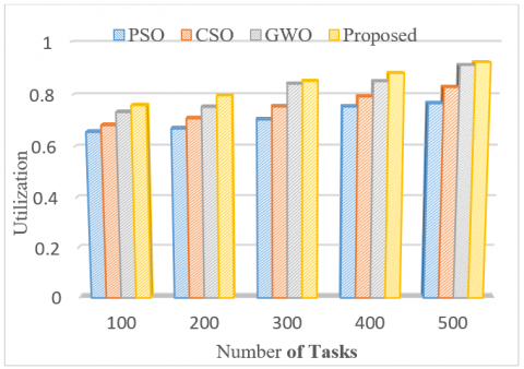
The results of the experiment prove to minimize the expense of cloud users while using cloud resources. The proposed approach efficiently utilizes the available resources impacting in reducing the cost. Figure 9 and Figure 10 depict the average resource utilization values which occupy the values between 0 to 1, and are calculated using the Eq. (8).
The simulation is performed for both scenarios by varying task numbers from the range 100-500. The results of the proposed method is compared with PSO, CSO and GWO algorithms.
As mentioned, the goal of the proposed work is to maximize resource utilization in the cloud. Through the experiment, it is found that in case of scenario-1, the utilization increases with an increase in the number of tasks but it is not the same during the random arrival of tasks as seen in scenario-2. It is perceived through simulation that in both the scenarios, the utilization value obtained by the proposed method is always higher than the other three algorithms. When compared with PSO, CSO and GWO, the proposed method produces 10.26%, 7.63%, 2.61% of upgradation in the utilization rate in scenario-1, likewise 8.76%, 6.14%, and 2.45% in case of scenario-2. The result proves to benefit the cloud providers by maximizing the revenue in the cloud environment. Overall the experimental results and analysis prove that the proposed method achieves the goal of minimizing makespan and cost while maximizing the utilization of resources.
Table 4 shows the resource utilization by the different types of VM’s in both scenario-1 and scenario-2. The results depict the actual usage of four different types of VM’s for varying task numbers from 100-500.
The obtained results help the service providers to create the actual number of VM’s required for task execution. Having prior knowledge of the type of tasks in the queue combined with the outcome of the proposed work offers the service providers the knowledge of the type of VM’s required for the execution of tasks.
In this paper, a three-stage strategy for solving multi-objective optimal task scheduling and resource allocation problems in the cloud is proposed. The proposed algorithm reduces makespan time and cost while increasing resource utilization.
The work categorizes incoming tasks into various categories based on resource demand and execution time. The tasks that have been classified are then queued separately. Similarly, VMs with varying resource capacities are created and queued distinctly. Using the proposed optimization task scheduling and allocation algorithm, the classified tasks are then mapped to the most appropriate VM type. The results of the experiments show that the proposed method outperforms the existing methods. More effort might be focused on testing with real datasets and the study could be broadened to investigate in an actual cloud system to evaluate its performance.
[1] Manvi, S.S., Shyam, G.K. (2014). Resource management for Infrastructure as a Service (IaaS) in cloud computing: A survey. Journal of Network and Computer Applications, 41: 424-440. https://doi.org/10.1016/j.jnca.2013.10.004
[2] Yousafzai, A., Gani, A., Noor, R.M., Sookhak, M., Talebian, H., Shiraz, M., Khan, M.K. (2017). Cloud resource allocation schemes: Review, taxonomy, and opportunities. Knowledge and Information Systems, 50(2): 347-381. https://doi.org/10.1007/s10115-016-0951-y
[3] Masdari, M., Gharehpasha, S., Ghobaei-Arani, M., Ghasemi, V. (2020). Bio-inspired virtual machine placement schemes in cloud computing environment: taxonomy, review, and future research directions. Cluster Computing, 23(4): 2533-2563. https://doi.org/10.1007/s10586-019-03026-9
[4] Anupama, K.C., Nagaraja, R., Jaiganesh, M. (2019). A perspective view of resource-based capacity planning in cloud computing. In 2019 1st International Conference on Advances in Information Technology (ICAIT), pp. 358-363. https://doi.org/10.1109/ICAIT47043.2019.8987357
[5] Domanal, S.G., Guddeti, R.M.R., Buyya, R. (2017). A hybrid bio-inspired algorithm for scheduling and resource management in cloud environment. IEEE Transactions on Services Computing, 13(1): 3-15. https://doi.org/10.1109/TSC.2017.2679738
[6] Ding, Z., Tian, Y.C., Tang, M., Li, Y., Wang, Y.G., Zhou, C. (2019). Profile-guided three-phase virtual resource management for energy efficiency of data centers. IEEE Transactions on Industrial Electronics, 67(3): 2460-2468. https://doi.org/10.1109/TIE.2019.2902786
[7] Albert, P., Nanjappan, M. (2020). An efficient kernel FCM and artificial fish swarm optimization-based optimal resource allocation in cloud. Journal of Circuits, Systems and Computers, 29(16): 2050253. https://doi.org/10.1142/S0218126620502539
[8] Jiang, C., Duan, Y., Yao, J. (2019). Resource-utilization-aware task scheduling in cloud platform using three-way clustering. Journal of Intelligent & Fuzzy Systems, 37(4): 5297-5305. https://doi.org/10.3233/JIFS-190459
[9] Mishra, A.K., Hellerstein, J.L., Cirne, W., Das, C.R. (2010). Towards characterizing cloud backend workloads: insights from google compute clusters. ACM SIGMETRICS Performance Evaluation Review, 37(4): 34-41. https://doi.org/10.1145/1773394.1773400
[10] Anupama, K.C., Shivakumar, B.R., Nagaraja, R. (2021). Resource utilization prediction in cloud computing using hybrid model. International Journal of Advanced Computer Science and Applications. https://doi.org/10.14569/issn.2156-5570
[11] Pang, S., Li, W., He, H., Shan, Z., Wang, X. (2019). An EDA-GA hybrid algorithm for multi-objective task scheduling in cloud computing. IEEE Access, 7: 146379-146389. https://doi.org/10.1109/ACCESS.2019.2946216
[12] Li, J.Q., Han, Y.Q. (2020). A hybrid multi-objective artificial bee colony algorithm for flexible task scheduling problems in cloud computing system. Cluster Computing, 23(4): 2483-2499. https://doi.org/10.1007/s10586-019-03022-z
[13] Sanaj, M.S., Prathap, P.J. (2020). Nature inspired chaotic squirrel search algorithm (CSSA) for multi objective task scheduling in an IAAS cloud computing atmosphere. Engineering Science and Technology, an International Journal, 23(4): 891-902. https://doi.org/10.1016/j.jestch.2019.11.002
[14] Jacob, T.P., Pradeep, K. (2019). A multi-objective optimal task scheduling in cloud environment using cuckoo particle swarm optimization. Wireless Personal Communications, 109(1): 315-331. https://doi.org/10.1007/s11277-019-06566-w
[15] Natesan, G., Chokkalingam, A. (2019). Optimal task scheduling in the cloud environment using a mean grey wolf optimization algorithm. International Journal of Technology, 10(1): 126-136. https://doi.org/10.14716/ijtech.v10i1.1972
[16] Natesan, G., Chokkalingam, A. (2020). An improved grey wolf optimization algorithm based task scheduling in cloud computing environment. Int. Arab J. Inf. Technol., 17(1): 73-81. https://doi.org/10.34028/iajit/17/1/9
[17] Sheetal, A.P., Ravindranath, K. (2019). Priority based resource allocation and scheduling using artificial bee colony (ABC) optimization for cloud computing systems. International Journal of Innovative Technology and Exploring Engineering, 8(6): 39-44. https://doi.org/10.35940/ijitee
[18] Mohammadzadeh, A., Masdari, M., Gharehchopogh, F. S., Jafarian, A. (2021). Improved chaotic binary grey wolf optimization algorithm for workflow scheduling in green cloud computing. Evolutionary Intelligence, 14(4): 1997-2025. https://doi.org/10.1007/s12065-020-00479-5
[19] Sreenu, K., Malempati, S. (2018). FGMTS: fractional grey wolf optimizer for multi-objective task scheduling strategy in cloud computing. Journal of Intelligent & Fuzzy Systems, 35(1): 831-844. https://doi.org/10.3233/JIFS-17148
[20] Sreenu, K., Malempati, S. (2019). MFGMTS: Epsilon constraint-based modified fractional grey wolf optimizer for multi-objective task scheduling in cloud computing. IETE Journal of Research, 65(2): 201-215. https://doi.org/10.1080/03772063.2017.1409087
[21] Marahatta, A., Pirbhulal, S., Zhang, F., Parizi, R.M., Choo, K.K.R., Liu, Z. (2019). Classification-based and energy-efficient dynamic task scheduling scheme for virtualized cloud data center. IEEE Transactions on Cloud Computing, 9(4): 1376-1390. https://doi.org/10.1109/TCC.2019.2918226
[22] Zhang, P., Zhou, M. (2017). Dynamic cloud task scheduling based on a two-stage strategy. IEEE Transactions on Automation Science and Engineering, 15(2): 772-783. https://doi.org/10.1109/TASE.2017.2693688
[23] Zuo, L., Dong, S., Shu, L., Zhu, C., Han, G. (2016). A multiqueue interlacing peak scheduling method based on tasks’ classification in cloud computing. IEEE Systems Journal, 12(2): 1518-1530. https://doi.org/10.1109/JSYST.2016.2542251
[24] Bezdan, T., Zivkovic, M., Bacanin, N., Strumberger, I., Tuba, E., Tuba, M. (2022). Multi-objective task scheduling in cloud computing environment by hybridized bat algorithm. Journal of Intelligent & Fuzzy Systems, 42(1): 411-423. https://doi.org/10.3233/JIFS-219200
[25] Zuo, L., Shu, L., Dong, S., Zhu, C., Hara, T. (2015). A multi-objective optimization scheduling method based on the ant colony algorithm in cloud computing. IEEE Access, 3: 2687-2699. https://doi.org/10.1109/ACCESS.2015.2508940
[26] Masadeh, R., Sharieh, A., Mahafzah, B. (2019). Humpback whale optimization algorithm based on vocal behavior for task scheduling in cloud computing. International Journal of Advanced Science and Technology, 13(3): 121-140.
[27] Lavanya, M., Shanthi, B., Saravanan, S. (2020). Multi objective task scheduling algorithm based on SLA and processing time suitable for cloud environment. Computer Communications, 151: 183-195. https://doi.org/10.1016/j.comcom.2019.12.050
[28] Reiss, C., Tumanov, A., Ganger, G.R., Katz, R.H., Kozuch, M.A. (2012). Heterogeneity and dynamicity of clouds at scale: Google trace analysis. In Proceedings of the Third ACM Symposium on Cloud Computing, pp. 1-13. https://doi.org/10.1145/2391229.2391236
[29] Mirjalili, S., Mirjalili, S.M., Lewis, A. (2014). Grey wolf optimizer. Advances in Engineering Software, 69: 46-61. https://doi.org/10.1016/j.advengsoft.2013.12.007
[30] Mittal, N., Singh, U., Sohi, B.S. (2016). Modified grey wolf optimizer for global engineering optimization. Applied Computational Intelligence and Soft Computing. https://doi.org/10.1155/2016/7950348
[31] Calheiros, R.N., Ranjan, R., Beloglazov, A., De Rose, C. A., Buyya, R. (2011). CloudSim: A toolkit for modeling and simulation of cloud computing environments and evaluation of resource provisioning algorithms. Software: Practice and Experience, 41(1): 23-50. https://doi.org/10.1002/spe.995