Manthena Narasimha Raju* | Kumaran Natarajan | Chandra Sekhar Vasamsetty
© 2022 IIETA. This article is published by IIETA and is licensed under the CC BY 4.0 license (http://creativecommons.org/licenses/by/4.0/).
OPEN ACCESS
The image classification of remote sensing (RS) plays a significant role in earth observation technology using RS data, extensively used in the military and civic sectors. However, the RS image classification confronts substantial scientific and practical difficulties because of RS data features, such as high dimensionality and relatively limited quantities of labeled examples accessible. In recent years, as new methods of deep learning (DL) have emerged, RS image classification approaches using DL have made significant advances, providing new possibilities for RS image classification research and development. Most of the researchers are using CNN to classify remote sensing images, but CNN alone problem with sequence data processing. But to get some sense out of the classification of remote sensing images. To avoid this in this paper, we use the CNN-LSTM model. The model performed ineffective classification of remote sensing images; the experimental results show that the proposed model is effective in classifying remote sensing images.
remote sensing, deep learning, CNN, LSTM, image classification, SIRI-WHU data
If you're interested in learning more about how remote sensing may help you classify scenes, you'll want to have a look at the Remote Sensing Scene Classification section [1]. Data from remote sensing images is crucial for understanding. The issue may be used in a number of areas, such as catastrophe monitoring and vegetation mapping, land resource management and urban planning, and traffic. Many distant sensors are gathering data with unique characteristics due to recent advancements in Earth observation technology, including remote sensing [2-6] technologies. It becomes difficult or perhaps impossible to manually analyze the data after it has been gathered since it is so vast and complicated. For example, remote sensors are frequently used to deliver data that is multi-source, multi-temporal, and multi-scale in nature.
In contrast, manually exploring them and extracting valuable information from them would be excessively time-consuming, and the performance would suffer. Therefore, the remote sensing research community has been concentrating its efforts in recent years on developing efficient techniques for processing remote sensing pictures [7-9] in combination with physics. Many scholars are interested in remote sensing, and there has been considerable development in this area. The picture below shows how quickly image processing methods for enhancement, analysis, and comprehension are developing. It is a well-known fact that there are still numerous difficulties to overcome in remote sensing, which stimulates new efforts and innovations to comprehend remote sensing pictures via image processing better.
Color and form are used in most prior approaches, or mid-level holistic picture representations [10-11] created by encoding hand-crafted visual characteristics are used. Computer vision has lately been transformed by Deep CNN, which has made significant advances in the domains like picture classification [12], object detection/segmentation [13-15], and action identification [16-19]. Neural networks that learn by watching data are known as DCNNs. The use of deep learning techniques in satellite image analysis, such as aerial scene classification [20] and hyperspectral picture analysis [21-25], has been similarly successful. As a general rule, DCNN takes a fixed-size picture as input and processes it via a convolution sequence, local normalization, and (termed as layers). These in-depth features may be utilized for several applications related to vision [26], which includes categorization of remote sensing scene] in a CNN [27] fully connected (FC) final layers. It's common for deep convolutional neural networks to be trained using data from the vast ImageNet dataset, a collection of RGB pixel values. When it comes to feature extraction in categorizing the scenes of remote sensing, these CNNs, which have been already trained on the dataset of ImageNet, are used by most current techniques. Unresolved research questions include studying various color spaces and integrating these color spaces for remote sensing scene classification. When it comes to vehicle color identification, He et al. [28] investigated the use of several color spaces; when it comes to super image resolution, Tang et al. [29] looked at the usage of YCbCr and RGB color channels in face recognition; Tang et al. [30] also proposed collaborative facial color feature learning approach that covered a variety of color spaces and included This study investigates a variety of color properties within the context of a deep learning framework for classification of scenes of remote sensing.
A lot of research was done before deep learning on the effects of different color features on object recognition and detection. When combined convolutional neural networks (CNNs) and long short-term memory (LSTMs) [31] are connected, sequential data classification system is created.
Because of this, most remote sensing scene classification techniques utilize a DCNN [32-36] that has previously been trained to identify an image. This approach, however, will run into the built-in problem of generating a high-dimensional final image representation when combining activations from several deep-color CNN. An effective classification system may be created by combining the properties of CNN with those of remote sensing images. The SIRI-WHU data collection is used throughout this paper. The rest of the article is organized as follows: On section two, you'll see the findings of existing models, as seen in Section 3, the suggested model is shown. On section 4, you'll find the details of the experiment, and on section 5, you'll find a summary.
Inspired by the capacity of human vision to identify items based on the highlights, which attracts the viewer's attention towards the object while disregarding the backdrop, the salient object identification technique is used to discover salient things. The salient model must captivate their attention to attract the attention of grasping items and complete segmentation of the objects [18]. Top-down and bottom-up techniques of salient item identification are used to detect salient objects, respectively. The bottom-up approach focuses on distinguishing between things in the background and those in the forefront in visual situations. On the other hand, top-down methods emphasize items unique to a specific category within visual sceneries.
According to Zhang et al. [19], there are two components to the salient object identification model. A patch-level cue exploration model and an object-level cue exploration model make up the model. As an initial stage, the objectless approach is used to identify the coarsely localized positions of the dominant feature of the image. If you want to know how well colors are dispersed in a space, you may use variance to estimate how compact it is. However, it didn't matter that the model did well in photos with a more plain background. For pictures with a conspicuous object and an environment that share a similar shade of color, this algorithm does not perform as well. As a result; it must be capable of extracting the regions and the objects that are distinct from one another in the image to enhance salient object.
Deep learning was utilized in Ref. [20] to concentrate on the layered skip structure, which was previously unknown. They developed a novel technique by including the holistically layered edge detector architecture, connections that are short in the skip-layer for the salient have been investigated, which was previously unexplored (HED). The VGGNet model and the HED model served as the basis for their proposed design. The combined characteristics from both the shallow and deep side outputs (salient regions) (low-level features) to get the best results. The architecture comprises interconnected phases, namely, the salient locating stage and the details refining stage, respectively. A top-to-bottom technique is introduced in the next step after the salient stage has identified salient areas in the picture and the clear view has been identified. Creating short connections between the two layers is necessary to forecast the salient items better. This results in an accurate and dense saliency map since the characteristics of both levels may be utilized to improve the prediction of the salient objects.
In an image, a method known as objectless detection creates many bounding boxes for every object possible without considering the item's category. Objectively, our goal is to provide a metric that may be used to generate candidate proposal ideas for consideration. The confidence score determines a proposal's inclusion or exclusion of an item. Two kinds of deep network object identification frameworks exist free and regional-based methods. The success of both region-free and region-based techniques [19] led to the development of a methodology [20] that integrates the best features of both methods. Several factors went into this, but the two most significant were multiscale localization and harmful space mining. In the case of localization that can be multiscale, there is a chance for objects to be discovered at any place on the image; authors have to consider all the locations while performing the object detection; on the other hand, it is recommended to utilize a reverse connection so that the objects may be recognized on the proper Convolutional feature-maps are subjected to an objectless prior phase during the training phase, which helps to decrease searching time for objects by reducing object search space. The Reverse connection with objectless previous networks architecture may be used to identify objects end-to-end with high precision. Convolutional layers are used to gather semantic information, which is then used in conjunction with reverse connections to create an objectless prior, which serves as a roadmap for searching for objects inside an image. Last but not least, the multitask loss function is used to complete the optimization process.
It's been demonstrated that data augmentation and harmful mining methods may help increase item detection accuracy [21]. To prevent exhaustingly looking for large sliding windows, there is a growing need for rapid object identification, such as moving cars, requiring fewer candidate windows to avoid exhaustingly searching for moving cars. One research suggested that the quality of the blind proposal must be improved by utilizing Union-Over-Intersection and Representation and Local Linear Regression (DORLLR) for Intersection-Over-Union to be used (IOU).
When employed in real-time object detection [22], it may be utilized to evaluate the quality of a sliding window that generates suggestions for the object detection task. Many attempts have been made to enhance the quality of the proposals via the use of blind estimates, and these efforts have proven fruitful. There are two possible explanations for the blind quality proposal evaluation. Because the foreground regions are believed to have more information than the background areas. It is regarded as a background and foreground segmentation problem when it comes to blind proposal quality. That's all it does. The segmentation method differentiates between the proposal quality at the back and the proposal quality. Instead of looking at scores and rankings based on particular visual cues, the first technique looks at the scores and ranks of the window function. An evaluation model for blind proposal quality (BPQA) has been created due to these factors to choose a greater number of proposals according to (BPQA). Both deep objectless representation and local linear regression are used during training. CNN-based feature extraction is utilized to mention the details of the deep objectless, and the local linear regression model is used to guess the quality of each recommendation.
In research [23], the model named hierarchical objectless network model was developed, which can identify object and proposal creation, among other things. They considered the most important aspects of object identification, such as accuracy, multi-scale, and computing cost, while developing their model. The model operates in three stages, with the CNN extracting the features from the picture in the first stage. The last step in which the stripe objectless is used to cut down the list of potential recommendations. It predicts a saliency map that may be used to search for objects. The Objectless stripes offer border objectless, in-out objectless, and in-out objectless, all contributing to the model's accuracy. They provide an object border and a score regarding the confidence in the suggested placement locations. Vertical and horizontal stripes have been added to the proposal to show the object border probability or object itself appearing in the vertical and the horizontal lines. To get high-level semantic information, it is essential to reverse the sequence of the deep and shallow convolutional layers. As a result of these qualities, a wide variety of resolution information is available for objects when seen at. Using just one saliency map, less memory is utilized, and less computation time is required.
Shen et al. [35] proposed a model for timeseries remote sensing pictures, we suggested a semi-supervised convolutional Long Short-Term Memory neural network (SemiLSTM) that was verified on three data sets with various time distributions in this research. By using a limited number of labelled samples in conjunction with a large number of unlabeled samples, it is possible to accomplish accurate and automatic land cover categorization. Aside from that, it is a very reliable classification technique for timeseries optical pictures with cloud covering, which minimises the need for cloudless remote sensing images and may be used broadly in places that are often hidden by clouds, such as subtropical areas.
Unnikrishnan et al. [36] proposed a two-band AlexNet architecture with a decreased number of filters was used to train the model in this study, and high-level features derived from the tested model were able to correctly categorise the various land cover classes available in the dataset. A comparison is made between the suggested architecture and a benchmark, and estimates are made on the outcomes in terms of accuracy, precision, and the total number of trainable parameters.
Most of the existing literature works are concentrated on classification of remote sensing images based on different deep learning models. And CNN model is used for classification of images it has a drawback of letting few features. If we consider all features will give better classification results.
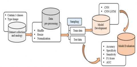
The full method for detecting things in a scene is shown in Figure 1, which is broken into many phases. It was necessary to submit raw remote sensing images to the preprocessing pipeline before they could be processed in the final processing pipeline. Data resizing, shuffling, and normalisation operations were performed on the data in the preprocessing channel. Following that, the preprocessed data set is separated into two parts: a training set and a large number of testing instances. Following the training data, we trained the CNN and CNN- We estimated the accuracy and loss for each phase of training. The system's performance was evaluated using measures such as sensitivity, accuracy, AUC based on ROC, confusion matrix, and F1-score to establish its effectiveness.
Figure 1. Proposed model architecture
3.1 CNN model
Backpropagation is the only method for getting all the parameters trained by their weights and biases in a convolutional neural network. Here's a quick rundown of what the algorithm is all about. In hidden layers, the function of cost concerning each unique training. For, example (x, y) may be expressed as follows:
$J(Q, \theta ; e, f)=\frac{1}{2}\|h y, \theta(e)-f\|^{2}$
Now, errors period A to the layer P, the equation is given as:
$A^{(P)}=\left(\left(Q^{(P)}\right)^{B} A^{(P+1)}\right) \cdot i^{\prime}\left(a^{(1)}\right)$
where the error for A(P+1)th layer is (A+1) whose cost function is J(Q, θ;e,f). i(a((1))) represents the derivative of activation function.
$\nabla y^{(P)} J(Q, \theta ; e, f)=A^{(P+1)}\left(j^{(P+1)}\right)^{B}$
$\nabla \theta^{(P)} J(X, \theta ; e, f)=A^{(P+1)}$ Where I is information, such that i((1)) is the information for the 1st layer (it is the correct input) and i((L)) is the information for the L-th layer.
The calculation for error of the sub-sampling layer Error is as:
$\Delta s^{(P)}=$ unsample $\left(\left(W_{S}^{(L)}\right)^{B} A_{K}^{(P+1)}\right) \cdot h^{\prime}\left(a_{S}^{(P) \mid}\right)$
In this case, q represents the number of filters in the layer. If mean pooling is utilized, the mistake must be cascaded oppositely in the subsampling layer. For example, when mean pooling is employed, upsampling equally shares the error for the preceding input unit. Finally, the gradient concerning the feature maps:
$\begin{aligned} \nabla y_{m}{ }^{(P)} n(X, \theta ; e, f) & \\ &=\sum_{b-1}\left(i_{t}^{(P)}\right) \\ & * \operatorname{rot} 90\left(A_{m}{ }^{(P+1)}, 2\right) \end{aligned}$
$\nabla \theta_{m}^{(P)}(X, \theta ; e, f)=\sum_{i, j}\left(A_{s}^{(P+1)}\right)_{i, j}$.
Algorithm
Backpropagation Algorithm in CNN
3.2 LSTM model
The following are the primary components of the LSTM unit:
$a_{t}=\tanh \left(X^{2} r_{b}+D^{2} i_{b-1}+d_{a}\right)$
$j_{b}=\sigma\left(X^{j} r_{b}+D^{j} i_{b-1}+d^{j}\right)$
From this process, LSTM learns how to re-establish the contents of its memory when they become obsolete and can no more serve a useful purpose. In such a case, the network would have to start processing a new set of instructions from scratch by employing a sigmoid activation, the forget gate, which is rt and ht1, activates inputs with weighted inputs. Once multiplied by the previous time step, it gives us the result jd. This allows us to delete any unnecessary memory content.
$v_{b}=\sigma\left(X^{v} r_{b}+D^{v} i_{b-1}+d_{v}\right)$
There are four types of memory cells: CEC, which has a repeating edge with unit weight, as well as an unweighted. By eliminating the unnecessary information (if any) from the preceding time step and accepting correct information (if any) from the present input, it is feasible to compute the current cell state sb.
$u_{b}=\sigma\left(X^{u} t_{d}+D^{u} i_{b-1}+d^{u}\right)$
Output gate: LSTM unit's output gate takes the weighted sum of xt and ht1 and uses the sigmoid activation to coordinate the data sent out from LSTM.
$h_{b}=a_{b} \odot j_{b}+h_{b-1} \odot v_{b}$
Output: To calculate the output of the LSTM unit (ht), the cell state st must be sent through an inverter (tanh) and multiplied by the output gate (out). It is possible to describe the operation of the LSTM unit using a series of equations similar to the following.
$i_{b}=\tanh \left(h_{b}\right) \bigodot u_{b}$
(1) The data needed for CNN-LSTM training must be entered first (see step one).
(2) Data standardization: As we have a significant gap in the data, the z-score standardization technique is used to normalize the input data to improve the model's training performance. The formula for this method is as follows:
$k_{i}=\frac{r_{j}-\bar{r}}{h}$
$r_{i}=k_{j} * h+\bar{r}$
If the standardized value (Yi), data taken as input (xi) is the average, and s represents the standard deviation of input data (xi) is the average and s means standard
(3) The biases and weights of each layer of the CNN-LSTM should be set to their initial values.
(4) A succession of feature extraction layers is applied to the input data before being transferred to the final convolution and pooling layers.
(5) It's also possible to use an LSTM algorithm to compute the CNN layer's output data, which can then be used to determine the output value.
(6) A comparison is made in step 6 of this process between the value generated computed by the layer that produces output and the actual number of the group data, and the inaccuracy is determined.
(7) This error is found when the output value computed by the output layer is compared to the actual value of the group.
(8) Error in the calculation: Eighteen) the forecasting must finish a certain number of cycles, the weight must be below a specific threshold, and the forecasting miserror rate must be below a certain point. Otherwise, the procedure will continue to step 9 if one or more conditions for completion are met. If one of the criteria for completion is met, training is complete, the CNN-LSTM network is updated, and step 10 is Backpropagation of computed errors.
(9) The biases and weights of every layer are updated, then go to step 4 to continue training the network.
(10) The forecasting model is saved.
(11) Input data: enter the data that will be used in the forecasting process, if any.
(12) Standardization of input data: The input data is standardized by a formula (8).
(13) To forecast, feed the standardized data into the CNN-LSTM trained model, and you'll get a predicted value.
(14) The model of CNN-LSTM generates a standardized value as an output, which is subsequently returned to its original value. Using the formula below (9). Where is the standard deviation of data, and x is the average value of input data.
(15) Finalise the forecasting process by presenting the corrected results.
DATASET
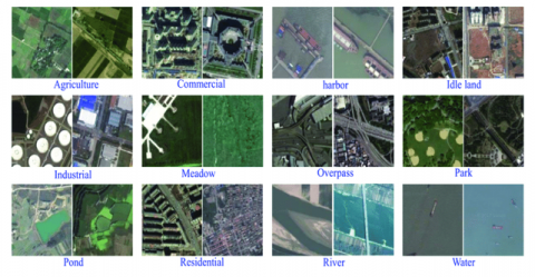
The RSIDEA group has compiled a collection of Google images of China's major cities (Remote Sensing Intelligent Data Retrieval, Interpretation, and Application).
In all, SIRI-WHU has 2,400 pictures and 12 situations. With a spatial resolution of 2 m, each class contains 200 images scaled at 200 pixels [29]. In addition to agriculture, enterprises, harbors [30], idle soil, production, wildlife, parks, and residential wetlands, the 12 land-use groups also include water and residential wetlands. Sample of 12 class Google image dataset of SIRI-WHU: (a) water; (b) river; (c) residential; (d) pond; (e) park; (f) overpass; (g) meadow; (h) industrial; (i) idle land; (j) harbor; (k) commercial; (l) agriculture. Here Figure 2 represents sample images from SIRI-WHU data set.
Figure 2. Images from SIRI-WHU data set
The positive true (e), positive false (f), negative true (g), or negative false(h) prediction are all possible outcomes in a binary classification issue (h). Where e indicates instances that are positive and expected to be positive, f denotes positive situations, and they are predicted to be negative, g means conditions that are negative and anticipated to be harmful, and h denotes problems that are negative and expected to be positive.
The most straightforward way to assess classification performance is to look at accuracy, the ratio of the number of adequately guessed situations to the total number of predicted instances. Then, using the language that has been presented, accuracy A may be calculated using the equation:
Accuracy is easy to understand, and it is used for both binary and multiple-class classification problems. However, accuracy could give an unfair representation of classification performance in imbalanced data sets. For example, in a binary classification problem where 90% of the samples are of the same class, simply assigning all cases to that class would already achieve an accuracy of 90%.
Therefore, we introduce three other metrics, which will be used to assess the per-class classification performance: precision, recall, and the F1-score. Accuracy indicates how many of the positive predicted cases are correctly expected, and recall expresses the fraction of all positive cases which are correctly predicted. These metrics are captured within the F1 metric, the harmonic mean of precision and recall. Precision (P), memory (R), and the F1-score (F1) are obtained by respectively:
Accuracy= (e+f)/(e+f+g+h)
Sensitivity= e/(e+h)
Specificity=f/(f+g)
F1-score=(2*e)/(2*e+g+h)
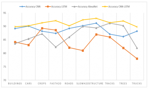
Figure 3. Accuracy
There are a lot of data points that can be appropriately calculated out of all the data. It's a little more complicated than that. Still, the number of true positives and real negatives is computed as dividing the number of positives true by the total number of positives actual. Positive, adverse facts are counted separately, with positive and negative falsehoods and negative truths separated. As you can see in Figure 3, the SIRI-WHU data set has an accuracy of identifying objects on top of that, the proposed CNN-LSTM and current models are differentiated to find the accuracy of object identification in the SIRI-W In Figure 3, we can see how well suggested and recent models have fared in terms of detecting. As a result, the presented model is more accurate in detecting the items than current.
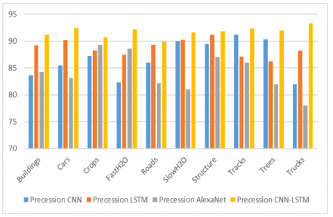
Figure 4. Precession
When it comes to pattern detection (also known as machine learning), accurate information (also known as positive predictive value) is the percentage of relevant examples among the retrievals. In contrast, rescue (sensitivity) fragments all related instances found. The precession of objects detected in SIRI-WHU data collection is shown in Figure 4. Besides, the suggested and existing models with various things are used to assess the precession of the detection of objects in the SIRI-WHU data set. A comparison between suggested and current models may be seen in Figure 4. The suggested model outperforms the current one in terms of objective observation.
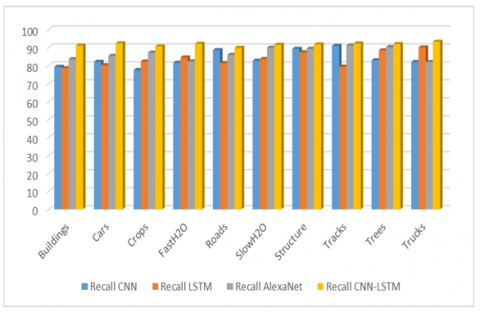
Figure 5. Recall
In statistics, a model's capacity to recognize every important instance in a dataset is known as a reminder. Remembrance may be defined as the addition of positive true, and harmful false. As you can see in Figure 5, the recall rate of identifying objects in the SIRI-WHU Apart from that, the proposed and current models with different things assess the recall of the SIRI-WHU dataset detection of objects remembrance. It is shown in Figure 5 that a recall of suggested and current models is carried out.
Figure 6. F-Score
Using the F-measure, the harmonic mean of accuracy and remembrance is determined. A single rating may be utilized to determine the output of the model and differentiate it to the consistency and reminder. The F1-score for identifying objects in the SIRI-WHU data set is shown in Figure 6. In addition, the proposed and current models with various items are used to assess the accuracy of the detection of objects in the SIRI-WHU data collection. A comparison of proposed and current models' F1 scores for detecting objects is shown in Figure 6.
With the purpose of categorising remote sensing photos using CNN-LSTM deep learning methods, we investigated the effect of colour in a CNN-LSTM deep learning system that was used to classify remote sensing photographs. Combining deep colour features with varied levels of information provides more efficient remote sensing scene categorization by expanding the number of categories available. The high dimensionality of deep colour feature fusion was also addressed, with the result that a dense final picture description was achieved without significant degradation in the five challenging remote sensing scene classification datasets that we used to evaluate the performance of our technique. Several of us believe that the strategy that has been described has shown to be really effective.
[1] Panetta, K. (2017). Gartner top 10 strategic technology trends for 2018-Smarter with Gartner. Gartner, Inc. https://www.gartner.com.
[2] Zhao, Z.Q., Zheng, P., Xu, S.T., Wu, X.D. (2019). Object detection with deep learning: A review. IEEE Transactions on Neural Networks and Learning Systems, 30(11): 3212-3232. https://doi.org/10.1109/TNNLS.2018.2876865
[3] Huang, T. (1996). Computer vision: Evolution and promise. 19th Cern Sch. Comput., pp. 21-25.
[4] Kamate, S., Yilmazer, N. (2015). Application of object detection and tracking techniques for unmanned aerial vehicles. Procedia Computer Science, 61: 436-441. https://doi.org/10.1016/j.procs.2015.09.183
[5] Pathak, A.R., Pandey, M., Rautaray, S. (2018). Application of deep learning for object detection. Procedia Computer Science, 132: 1706-1717. https://doi.org/10.1016/j.procs.2018.05.144
[6] Ouyang, W., Wang, X., Zeng, X., et al. (2015). DeepID-Net: Deformable deep convolutional neural networks for object detection. In Proceedings of the IEEE Conference on Computer Vision and Pattern Recognition, pp. 2403-2412. https://doi.org/10.1109/TPAMI.2016.2587642
[7] Pittaras, N., Markatopoulou, F., Mezaris, V., Patras, I. (2017). Comparison of fine-tuning and extension strategies for deep convolutional neural networks. In International Conference on Multimedia Modeling, pp. 102-114. https://doi.org/10.1007/978-3-319-51811-4_9
[8] TensorFlow. (2018). Available: https://www.tensorflow.org/.
[9] Keras. (2018). Available: https://keras.io/.
[10] Microsoft Cognitive Toolkit. (2018). Available: https://www.microsoft.com/en-us/cognitive-toolkit/.
[11] PyTorch. (2018). Available: https://pytorch.org/about/.
[12] Unsupervised Feature Learning and Deep Learning Tutorial. (2018). Available: http://ufldl.stanford.edu/tutorial/supervised/FeatureExtractionUsingConvolution/.
[13] Liang, M., Hu, X. (2015). Recurrent convolutional neural network for object recognition. In Proceedings of the IEEE Conference on Computer Vision and Pattern Recognition, pp. 3367-3375. https://doi.org/10.1109/CVPR.2015.7298958
[14] Girshick, R. (2015). Fast R-CNN. In Proceedings of the IEEE International Conference on Computer Vision, pp. 1440-1448. https://doi.org/10.1109/ICCV.2015.169
[15] LeCun, Y., Bengio, Y., Hinton, G. (2015). Deep learning. Nature, 521(7553): 436-444. https://doi.org/10.1038/nature14539
[16] Goodfellow, I., Bengio, Y., Courville, A. (2016). Deep Learning. MIT press.
[17] Han, J., Zhang, D., Cheng, G., Liu, N., Xu, D. (2018). Advanced deep-learning techniques for salient and category-specific object detection: A survey. IEEE Signal Processing Magazine, 35(1): 84-100. https://doi.org/10.1109/MSP.2017.2749125
[18] Borji, A., Cheng, M.M., Jiang, H., Li, J. (2015). Salient object detection: A benchmark. IEEE Transactions on Image Processing, 24(12): 5706-5722. https://doi.org/10.1109/TIP.2015.2487833
[19] Zhang, Q., Lin, J., Li, W., Shi, Y., Cao, G. (2018). Salient object detection via compactness and objectness cues. The Visual Computer, 34(4): 473-489. https://doi.org/10.1007/s00371-017-1354-0
[20] Hou, Q., Cheng, M.M., Hu, X., Borji, A., Tu, Z., Torr, P.H. (2017). Deeply supervised salient object detection with short connections. In Proceedings of the IEEE Conference on Computer Vision and Pattern Recognition, pp. 3203-3212. https://doi.org/10.1109/CVPR.2017.563
[21] Kong, T., Sun, F., Yao, A., Liu, H., Lu, M., Chen, Y. (2017). Ron: Reverse connection with objectness prior networks for object detection. In Proceedings of the IEEE Conference on Computer Vision and Pattern Recognition, pp. 5936-5944. https://doi.org/10.1109/CVPR.2017.557
[22] Wu, Q., Li, H., Meng, F., Ngan, K.N., Xu, L. (2017). Blind proposal quality assessment via deep objectness representation and local linear regression. In 2017 IEEE International Conference on Multimedia and Expo (ICME), pp. 1482-1487. https://doi.org/10.1109/ICME.2017.8019305
[23] Wang, J., Tao, X., Xu, M., Duan, Y., Lu, J. (2018). Hierarchical objectness network for region proposal generation and object detection. Pattern Recognition, 83: 260-272. https://doi.org/10.1016/j.patcog.2018.05.009
[24] Gopi, A.P., Naga Sravana Jyothi, R., Lakshman Narayana, V., Satya Sandeep, K. (2020).."Classification of tweets data based on polarity using improved RBF kernel of SVM. International Journal of Information Technology, 1-16. https://doi.org/10.1007/s41870-019-00409-4
[25] Girshick, R., Donahue, J., Darrell, T., Malik, J. (2014). Rich feature hierarchies for accurate object detection and semantic segmentation. In Proceedings of the IEEE Conference on Computer Vision and Pattern Recognition, pp. 580-587. https://doi.org/10.1109/CVPR.2014.81
[26] Erhan, D., Szegedy, C., Toshev, A., Anguelov, D. (2014). Scalable object detection using deep neural networks. In Proceedings of the IEEE Conference on Computer Vision and Pattern Recognition, pp. 2147-2154. https://doi.org/10.1109/CVPR.2014.276
[27] Kuo, W., Hariharan, B., Malik, J. (2015). Deepbox: Learning objectness with convolutional networks. In Proceedings of the IEEE International Conference on Computer Vision, pp. 2479-2487. https://doi.org/10.1109/ICCV.2015.285 PMid:25693659
[28] He, K., Zhang, X., Ren, S., Sun, J. (2016). Deep residual learning for image recognition. In Proceedings of the IEEE Conference on Computer Vision and Pattern Recognition, pp. 770-778.
[29] Tang, Y., Wang, J., Gao, B., Dellandréa, E., Gaizauskas, R., Chen, L. (2016). Large scale semi-supervised object detection using visual and semantic knowledge transfer. In Proceedings of the IEEE Conference on Computer Vision and Pattern Recognition, pp. 2119-2128. https://doi.org/10.1109/CVPR.2016.233
[30] Tang, Y., Wang, X., Dellandrea, E., Chen, L. (2016). Weakly supervised learning of deformable part-based models for object detection via region proposals. IEEE Transactions on Multimedia, 19(2): 393-407. https://doi.org/10.1109/TMM.2016.2614862
[31] Ren, S., He, K., Girshick, R., Sun, J. (2015). Faster R-CNN: Towards real-time object detection with region proposal networks. Advances in Neural Information Processing Systems. 39(6): 1137-1149. https://doi.org/10.1109/TPAMI.2016.2577031
[32] Zhou, P., Ni, B., Geng, C., Hu, J., Xu, Y. (2018). Scale-transferrable object detection. In proceedings of the IEEE Conference on Computer Vision and Pattern Recognition, pp. 528-537. https://doi.org/10.1109/CVPR.2018.00062
[33] Chu, W., Cai, D. (2018). Deep feature based contextual model for object detection. Neurocomputing, 275: 1035-1042. https://doi.org/10.1016/j.neucom.2017.09.048
[34] Fu, K., Gu, I. Y.H., Yang, J. (2018). Spectral salient object detection. Neurocomputing, 275: 788-803. https://doi.org/10.1016/j.neucom.2017.09.028
[35] Shen, J., Tao, C., Qi, J., Wang, H. (2021). Semi-supervised convolutional long short-term memory neural networks for time series land cover classification. Remote Sensing, 13(17): 3504. https://doi.org/10.3390/rs13173504
[36] Unnikrishnan, A., Sowmya, V., Soman, K.P. (2018). Deep AlexNet with reduced number of trainable parameters for satellite image classification. Procedia Computer Science, 143: 931-938. https://doi.org/10.1016/j.procs.2018.10.342