Halaguru Basavarajappa Basanth Kumar | Haranahalli Rajanna Chennamma*
© 2021 IIETA. This article is published by IIETA and is licensed under the CC BY 4.0 license (http://creativecommons.org/licenses/by/4.0/).
OPEN ACCESS
With the rapid advancement in digital image rendering techniques, allows the user to create surrealistic computer graphic (CG) images which are hard to distinguish from photographs captured by digital cameras. In this paper, classification of CG images and photographic (PG) images based on fusion of global features is presented. Color and texture of an image represents global features. Texture feature descriptors such as gray level co-occurrence matrix (GLCM) and local binary pattern (LBP) are considered. Different combinations of these global features are investigated on various datasets. Experimental results show that, fusion of color and texture features subset can achieve best classification results over other feature combinations.
appearance-based features, color, computer graphic images, feature fusion, photographic images, photo-realistic computer graphic images, texture
Recent development in computer graphics (CG) image rendering technology has made easy for the content creators to produce synthetic images which exhibits high photo-realism and hard to distinguish from photographic (PG) images by naked eyes. If such images are used illegitimately in journalism or forensic investigation, then it may cause serious threat to the society [1]. Therefore, classification of CG and PG images has become important research topic in the field of digital image forensics. Researchers have addressed this problem using classical machine learning and deep learning approaches with different perspectives in the past decade. However, the ability of computational techniques in classifying CG and PG images is still needs to be improved.
In this work, global features such as color and texture are extracted from an image as these features exhibit basic difference between CG and PG images efficiently. Support vector machine (SVM) classifier is used for classification.
The rest of this paper is outlined as follows: Section 2 introduces review of related works based on classical machine learning and deep learning approaches. Section 3 describes proposed method. Experimental results and performance analysis are given in Section 4. Further, conclusion is given in Section 5.
State-of-the-art techniques used to distinguish CG and PG images can be grouped into four categories depending on features selected for classification: camera characteristics, spatial features, geometric features and deep learning based techniques.
Camera characteristics: These features deal with inherent characteristics like photo response non-uniformity (PRNU) noise, chromatic aberration, color filter array (CFA) interpolation, etc., associated with digital camera.
Spatial features: Spatial features deal with the contents of an image. Features like histogram features, textural features, etc., are some examples of spatial features which describes image contents.
Geometric features: Geometric features deal with geometric properties such as edges, corners, blobs and so on of the image.
Deep learning techniques: These techniques learn features automatically from input image. Convolutional neural networks based deep learning is most widely used for classification tasks.
2.1 Techniques based on camera characteristics
Images produced by digital camera and computer graphic software tools usually undergo different creation processes. Based on this fact, Dehni et al. [2] presented a scheme by extracting the properties of residual images using wavelet based denoising filter. They found that each digital camera exhibits distinct noise pattern which cannot be found in computer graphics. Dirik et al. [3] proposed a technique based on two features: traces of demosaicking and chromatic aberration. Four new features are introduced to detect the presence of color filter array (CFA) interpolation. Mutual information between color channels is used to measure the misalignment. Khanna et al. [4] presented a technique based on the residual pattern noise present in digital cameras and scanners. Residual pattern noise exists in computer graphic images which does not have similar structure. These features are used for the classification of scanner, computer generated and digital camera images. Peng et al. [5] analysed the difference between image textures of PG images and PRCG images based on multifractal spectrum features of PRNU. 8 dimensions of multifractal features are extracted and an average classification accuracy of 98.99% is attained with a dataset containing 2000 PG images and 2000 PRCG images. Peng and Zhou [1] have analysed the effect of CFA interpolation on the local correlation of PRNU as it is used in the natural image generation. Maximum of histogram, difference of histogram and variance of histogram are calculated for RGB channels by extracting 9 feature dimensions. An average accuracy of 99.43% is obtained on a database containing 1200 computer graphic images and 1200 photographic images. Long et al. [6] presented a scheme based on binary similarity measure computed from PRNU in RGB channels. An average classification accuracy of 99.83% is achieved with 36 features by using 3000 PGs and 3000 CGs.
2.2 Techniques based on spatial features
Pan et al. [7] found that perceptual difference between CGs and PGs present in color and coarseness of images. Based on this fact, color difference is found using fractal dimension and coarseness is analysed using generalized dimension. An average accuracy of 91.2% is observed with a dataset of 3000 CGs and 3000 PGs. Wu et al. [8] employ histogram bins of first order and second order difference as features for classification of CG and PG images. Li et al. [9] extracted 59 dimensions of uniform gray-scale LBP features from the YCBCr model of each image, and an average classification accuracy of 98.3% is obtained using a dataset of 2455 CGs and 2455 PGs. Peng et al. [10] presented a novel scheme by analysing the differences between statistical and textural features. An accuracy of 97.89% and 97.75% are obtained for natural images and computer graphic images by using LIBSVM with 31 features on a dataset of 2400 images where each class contain 1200 images. Peng et al. [11] examined the differences in texture between residual images of natural images and computer graphics. Further, they investigated fitting degree of regression model. An average classification accuracy of 98.69% is obtained with 24 features on a dataset of 3000 PGs and 3000 CGs.
2.3 Techniques based on geometric features
Wang and Moulin [12] presented a wavelet-based statistical model for classification of PRCG and PG images. An average accuracy of 100% is attained with 144 features on a dataset of 4546 PG images and 3844 PRCG images. Chen et al. [13] proposed α-stable model to extract fractional lower order moments. Three-level wavelet decomposition is performed on RGB channels and 27 high frequency sub-bands are obtained. Performance of the scheme is evaluated on a dataset consisting 2000 images where each category contains 1000 images and an average accuracy of 81.85% is achieved. Zhang and Wang [14] proposed a method using imaging features and visual features extracted from wavelet sub-bands. Statistical features and cross correlation of wavelet coefficients from each sub-band are used as features. Fan et al. [15] proposed a modified contourlet transform for classification of CG and natural images. Four-level wavelet decomposition is applied to an image in HSV color space to extract statistical features. Highest classification accuracy of 93.51% is obtained for HSV color space and its image prediction error with 384 features by using a database of 800 CGs and 800 PGs. Birajdar and Mankar [16] use binary statistical image features by decomposing gray scale image into sub-bands using Harr wavelet transform. Relevant features are selected by using fuzzy entropy measure and an average accuracy of 87.72% is obtained with a dataset of 800 CGs and 800 PGs.
2.4 Techniques based on deep learning
Rahmouni et al. [17] proposed a stats-2L model with custom poling layer to extract statistical properties. Further, a weighted voting technique is employed to predict the image class of the entire picture. Best classification accuracy of 93.2% is observed using a dataset containing 1800 CGs and 1800 PGs. Yao et al. [18] employed several pre-defined filters to obtain sensor noise residuals and presented a five layer CNN framework to discriminate CG and PG images. Best performance model is obtained with three high pass filters and 100 % accuracy is achieved for full-size images. Chawla et al. [19] proposed five layer CNN model by employing some error prediction filters on to the special layer to ensure the correlation between pixels in CG and PG images. A weighted voting scheme is used to estimate the class probabilities and majority voting scheme is deployed to predict the label of original image. 100% accuracy attained for full-size images. Nguyen et al. [20] employed VGG19 pre-trained network model as a feature extractor. Output of first, second and third convolution layers are used as features and statistical pooling layer was constructed. Up to 100% accuracy was observed for a patch size of 256×256. He [21] employed two pre-trained network models namely, VGG19 and ResNet50 for classification of CG and PG images and evaluated their performances. An average accuracy of 96% is achieved on DSTok dataset consists of 4850 CGs and 4850 PGs. Experimental results show that ResNet50 is more accurate than VGG19.
From the above study, we found that, there is no benchmark and challenging CG and PG image dataset available which are created using latest technologies. Conventional machine learning approaches lacks generalization of techniques. In contrary, deep learning approaches involve high computational complexity due to large feature vector dimension.
In this work, we have introduced fusion of appearance-based features such as color and texture to classify CG and PG images and the contributions of this paper are as follows:
A dataset is created consisting of heterogeneous collection of computer graphic, photographic and photo-realistic computer graphic images.
Various combinations of color and texture features are analysed to select optimal subset of features which improves accuracy of the classification model.
Effectiveness of the classification model is assessed on Columbia dataset, DSTok dataset and two own datasets.
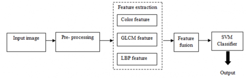
In this section, appearance-based features such as color and texture are used to classify CG and PG images. The detailed description of these features and SVM classifier used for classification is given below. Figure 1 shows different stages of image category classification.
Figure 1. Stages of image classification
3.1 Pre-processing
In image pre-processing stage, uniformity is maintained by resizing all CG and PG images to a dimension of 256×256 pixels. All these images are converted to grayscale for texture feature extraction.
3.2 Feature extraction
In this stage, we extract global features such as color and texture to classify CG and PG images. CG images are often exhibit high contrast when compared to PG images and coarseness of images appear smooth on CG images.
3.2.1 Color feature
Color feature describes two characteristics: total number of colors present in an image and distribution of colors spatially. In this work, mean and color percentage of RGB channels are considered. Given image is partitioned into 8 equal subblocks. Let Ch1, Ch2, Ch3 represents R, G, B channels. The mean value of each subblock for each channel is computed using Eq. (1).
$\overline{\mathrm{Ch}}_{\mathrm{i}}^{\mathrm{K}}=\frac{\sum \mathrm{ch}_{\mathrm{i}}^{\mathrm{K}}}{\text { No. of pixels in the respective subblock }}$ (1)
where, 1≤i≤8 and k=1,2,3.
Furthermore, percentage of each subblock for each channel is computed which yields degree of color component using equations from (2) to (4).
$P_{1, i}=\frac{\overline{C h}_{i}^{1}}{\text { Totalcolor }_\quad{i}} * 100$ (2)
$P_{2, i}=\frac{\overline{C h}_{i}^{2}}{\text { Totalcolor }_\quad{i}} * 100$ (3)
$P_{3, i}=\frac{\overline{C h}_{i}^{3}}{\text { TotalColor }_\quad{i}} * 100$ (4)
where, TotalColor $_{\mathrm{i}}=\overline{\mathrm{Ch}}_{\mathrm{i}}^{1}+\overline{\mathrm{Ch}}_{\mathrm{i}}^{2}+\overline{\mathrm{Ch}}_{\mathrm{i}}^{3}$ and i=1,2,3.
P1,i , P2,i and P3,i in the above equations corresponds to red, green and blue channels respectively. Mean value and color percentage of each subblock for each channel has yielded 48 dimensions of features [22].
3.2.2 Texture feature descriptors
Texture is the low-level visual feature which defines the image characteristics. Texture descriptors such as gray level cooccurrence matrix (GLCM) [23] and local binary pattern (LBP) [24] are adopted which are most widely used texture descriptors in image texture analysis.
(1) GLCM descriptor
GLCM texture descriptor is used to compute the spatial relationship among the pixels in an image. It is denoted by using a pair of parameters (Θ, d) where ‘Θ’ represents orientation and ‘d’ is the distance between two pixels. Rotational invariance is achieved by defining set of orientation parameters, usually 8 orientations are considered and they are separated by P/4 radians away.
Co-occurrence matrices are obtained using d=1 and Θ = 0 degree. 14 statistical measures (Table 1) described by Haralick et al. are computed from GLCM and used as feature descriptors. The equations containing the variable q(r, s) indicates a value at (r, s) position in GLCM. Feature vector consisting of 14 statistical measures obtained for the whole image.
(2) LBP descriptor
LBP is a local visual texture descriptor which labels every pixel in an image by comparing neighborhood of each picture element in an image and produces the binary sequence. The neighborhood of a pixel is represented as P number of neighbors within a circle of radius R. In this work, P=16 and R=1 are used. The result of a LBP of a picture element is given in Eq. (5) and f(p) is given in Eq. (6).
$\mathrm{LBP}_{\left(\mathrm{x}_{\mathrm{c}}, \mathrm{y}_{\mathrm{c}}\right)}=\sum_{\mathrm{n}=0}^{\mathrm{n}-1} \mathrm{f}\left(\mathrm{G}_{\mathrm{n}}-\mathrm{G}_{\mathrm{c}}\right) * 2^{\mathrm{n}}$ (5)
$f(p)=\left\{\begin{array}{lr}1, & \text { if } p \geq 0 \\ 0, & \text { Otherwise }\end{array}\right.$ (6)
Initially, Input image is partitioned into cells and each pixel of a cell is compared to its 16 neighbors along the circle of radius 1 in clock-wise direction. If a neighborhood pixel value is greater than the central pixel value then mark as 1. Else, mark as 0. From this, a binary sequence consisting of 16 digits is obtained. Histogram is computed over the cell for each number which has most frequently occurred. Using uniform-LBP, the feature vector is reduced to 243.
Table 1. Haralick features
|
Statistical measure |
Formula |
|
Energy |
$\sum_{\mathbf{r}} \sum_{\mathrm{s}}\{\mathrm{q}(\mathrm{r}, \mathrm{s})\}^{2}$ |
|
Contrast |
$\sum_{\mathrm{r}, \mathrm{s}}|\mathrm{r}-\mathrm{s}|^{2} \mathrm{q}(\mathrm{r}, \mathrm{s})$ |
|
Correlation |
$\sum_{\mathbf{r}, \mathrm{s}} \frac{\left(\mathrm{r}-\mu_{\mathrm{r}}\right)\left(\mathrm{s}-\mu_{\mathrm{s}}\right) \mathrm{q}(\mathrm{r}, \mathrm{s})}{\sigma_{\mathrm{r}} \sigma_{\mathrm{S}}}$ |
|
Variance |
$\sum_{\mathrm{r}} \sum_{\mathrm{s}}(\mathrm{r}-\mu)^{2} \mathrm{q}(\mathrm{r}, \mathrm{s})$ |
|
Homogeneity |
$\sum_{\mathrm{r}, \mathrm{s}} \frac{\mathrm{q}(\mathrm{r}, \mathrm{s})}{1+|\mathrm{r}-\mathrm{s}|}$ |
|
Sum average |
$\sum_{\mathrm{r}=2}^{2 \mathrm{P}_{\mathrm{g}}} \mathrm{rq}_{\mathrm{u}+\mathrm{v}}(\mathrm{r})$ |
|
Sum variance |
$\sum_{\mathrm{r}=2}^{2 \mathrm{P}_{\mathrm{g}}}(\mathrm{r}-\text { sum entropy })^{2} \mathrm{q}_{\mathrm{u}+\mathrm{v}}(\mathrm{r})$ |
|
Sum entropy |
$-\sum_{\mathrm{r}=2}^{2 \mathrm{P}} \mathrm{q}_{\mathrm{u}+\mathrm{v}}(\mathrm{r}) \log \left\{\mathrm{q}_{\mathrm{u}+\mathrm{v}}(\mathrm{r})\right\}$ |
|
Entropy |
$-\sum_{\mathrm{r}} \sum_{\mathrm{s}} \mathrm{q}(\mathrm{r}, \mathrm{s}) \log (\mathrm{q}(\mathrm{r}, \mathrm{s}))$ |
|
Difference entropy |
$-\sum_{\mathrm{r}=0}^{\mathrm{P}_{\mathrm{g}-1}} \mathrm{q}_{\mathrm{u}-\mathrm{v}}(\mathrm{r}) \log \left\{\mathrm{q}_{\mathrm{u}-\mathrm{v}}(\mathrm{r})\right\}$ |
|
Information measures of correlation |
$\frac{\text { HUV-HUV1 }}{\max \{\mathrm{HU}, \mathrm{HV}\}}$ $(1-\exp [-2.0(\mathrm{HUV} 2-\mathrm{HUV})])^{1 / 2}$ $\mathrm{HUV}=-\sum_{\mathrm{r}} \sum_{\mathrm{s}} \mathrm{q}(\mathrm{r}, \mathrm{s}) \log (\mathrm{q}(\mathrm{r}, \mathrm{s}))$ $\mathrm{HUV} 1=-\sum_{\mathrm{r}} \sum_{\mathrm{s}} \mathrm{q}(\mathrm{r}, \mathrm{s}) \log \left\{\mathrm{q}_{\mathrm{u}}(\mathrm{r}) \mathrm{q}_{\mathrm{v}}(\mathrm{s})\right\}$ $\mathrm{HUV} 2=-\sum_{\mathrm{r}} \sum_{\mathrm{s}} \mathrm{q}_{\mathrm{u}}(\mathrm{r}) \mathrm{q}_{\mathrm{n}}(\mathrm{s}) \log \left\{\mathrm{q}_{\mathrm{u}}(\mathrm{r}) \mathrm{q}_{\mathrm{v}}(\mathrm{s})\right\}$ |
|
Maximal correlation coefficient |
(Second largest eigen value of $Q)^{1 / 2}$ $Q(r, s)=\sum_{t} \frac{q(r, t) q(s, t)}{q_{u}(r) q_{v}(s)}$ |
(3) Feature fusion
Color and texture descriptors such as GLCM and LBP are fused at feature level. Different color and texture feature fusion are analysed to select best feature subset which produces optimal classification accuracy. Thus, the different feature combinations are: single feature (Color – 48 features, GLCM – 14 features and LBP – 243 features are extracted independently), two feature combination yields 3 sets of features (Color+GLCM – 62 features, Color+LBP – 291 features and GLCM+LBP – 257 features) and three feature combination yields only one set of feature (Color+GLCM+LBP – 305 features). A total of seven combinations are used for the classification of CG and PG images.
3.3 SVM classifier
Support vector machine [25] classifier is widely used supervised learning model for classification task. It is used to perform either linear or non-linear classification. When two classes could not be segregated with linear hyper-plane, kernel concept is used to classify non-linear data. Radial basis function kernel is used in our study. It is described as follows:
$\mathrm{K}\left(\mathrm{x}, \mathrm{x}^{1}\right)=\exp \left(-\frac{\left\|\mathrm{x}-\mathrm{x}^{1}\right\|^{2}}{2 \sigma^{2}}\right)$ (7)
where, x and x1 are the two samples, represented as feature vectors in some input space.
||x-x1||2 is the squared Euclidean distance between two feature vector points.
$k\left(x, x^{1}\right)=\exp \left(-\gamma\left\|x-x^{1}\right\|^{2}\right)$ (8)
where, $\gamma=\frac{1}{2 \sigma^{2}}$.
4.1 Dataset
Four datasets are used for the experimentation. A benchmark dataset – “Columbia Photographic Images and Photorealistic Computer Graphics Dataset” consists of 800 CG and PG images [26], “DSTok Dataset” comprises of 4850 CG images and 4850 PG images [27] and two own datasets namely, “JSSSTU CG and PG Image Dataset” contain 7000 CG images and 7000 PG images and “JSSSTU PRCG Image Dataset” includes 2000 photo-realistic computer graphics and 2000 PG images are taken from JSSSTU PG Image Dataset. PG images are captured from different camera models and also selected from other data sources such as INRIA [28], ICCV09 [29] McGill Calibrated Colour Image Database [30]. CG images are collected from various online sources. The contents of PG images cover a wide collection of indoor scenes, outdoor scenes, nature, objects, people, and buildings etc. CG images similarly involve diversified contents which includes photo-realistic images, non-photo-realistic images, and video gaming screenshots and so on.
4.2 Experimental setup
In pre-processing phase, all CG and PG images are rescaled to a dimension of 256×256 pixels which helps to maintain the uniformity during feature extraction from all the images. To extract GLCM and LBP texture features, CG and PG images are converted into grey levels apart from the color features. During feature extraction phase, color feature and texture features such as GLCM and LBP are extracted from CG and PG images resulting in 48, 14 and 243 features respectively. Classification is carried out based on these three features and their combinations using SVM classifier.
All datasets are randomly partitioned into different ratios of training and testing: 50:50, 70:30 and 80:20 respectively.
4.3 Experimental results
Effectiveness of the proposed classification model is assessed based on accuracy, precision, recall and f-score obtained from the confusion matrix.
The overall classification accuracy of the model is given by:
Accuracy $=\frac{\text { No. of correctly classified instances }}{\text { Total instances }} * 100$ (9)
Precision and recall are computed for each image class and are given in the Eqns. (10) and (11).
$P_{i}=\frac{\text { No. of correctly classified instances }}{\text { Total classified instances }}$ (10)
$\mathrm{R}_{\mathrm{i}}=\frac{\text { No. of correctly classified instances }}{\text { Total expected instances }}$ (11)
Macro average of the classes is computed as follows:
Precision $=\frac{\sum_{\mathrm{i}=1}^{\mathrm{n}} \mathrm{P}_{\mathrm{i}}}{\mathrm{n}}$ (12)
Recall $=\frac{\sum_{\mathrm{i}=1}^{\mathrm{n}} \mathrm{R}_{\mathrm{i}}}{\mathrm{n}}$ (13)
For i=1, 2, ..., n. Where, n = Number of image classes.
F-score is obtained from precision and recall is given by:
$\mathrm{F}-$ score $=\frac{2 \times \text { Precision } \times \text { Recall }}{\text { Precision }+\text { Recall }}$ (14)
Efficiency of the different feature extraction techniques and their combinations on various datasets under different training and testing ratios are tabulated. The overall accuracy of classification model on various datasets is shown in the Tables from 2 to 5.
From Table 2, it is found that, LBP feature descriptor has achieved best classification accuracy on Columbia Dataset for the training and testing ratio 70:30. From Tables 3 to 5, we can observe that, performance of the classification model increases when more than one feature is considered.
Best classification results attained for color, GLCM, LBP and feature fusion (color+GLCM+LBP) are tabulated in terms of accuracy, precision, recall and f-score on different datasets and are shown in the Tables from 6 to 9. From Table 6, maximum classification accuracy of 98.12% is obtained for LBP feature using Columbia Dataset with only 243 feature vector dimensions but f-score obtained for LBP and fusion of color, GLCM and LBP feature remains 0.98. From Tables 6 to 9, we found that the classification model yields best classification result for fusion of color, GLCM and LBP features when compared to independent features. F-score obtained for fusion of color and texture features on DSTok dataset, JSSSTU CG and PG Image Dataset and JSSSTU PRCG Image Dataset is 0.84, 0.90 and 0.83 respectively.
Seven feature subsets are analysed to select the best feature subset which produces optimal classification results in terms of f-score. From the above study, we found that, fusion of color, GLCM and LBP features yields best results when compared to other feature combinations. Fusion of three features has yielded low detection rate on DSTok Dataset and JSSSTU PRCG Image Dataset due to complex photo-realistic computer graphics images contained in these datasets.
Table 2. Classification accuracy on Columbia dataset using SVM classifier
|
Train-Test % |
Color |
GLCM |
LBP |
Color+GLCM |
Color+LBP |
GLCM+LBP |
Color+GLCM+LBP |
|
50-50 |
67.37 |
73.25 |
97.37 |
76.12 |
97.37 |
97.50 |
97.12 |
|
70-30 |
68.75 |
75 |
98.12 |
76.87 |
97.50 |
97.70 |
97.29 |
|
80-20 |
70.93 |
72.81 |
97.81 |
77.50 |
97.50 |
97.81 |
97.50 |
Table 3. Classification accuracy on DSTok dataset using SVM classifier
|
Train-Test % |
Color |
GLCM |
LBP |
Color+GLCM |
Color+LBP |
GLCM+LBP |
Color+GLCM+LBP |
|
50-50 |
69.95 |
70.53 |
76.51 |
76.04 |
81.52 |
79.11 |
81.87 |
|
70-30 |
69.58 |
70.48 |
78.07 |
76.32 |
82.26 |
79.65 |
82.37 |
|
80-20 |
70.30 |
72.11 |
76.95 |
75.77 |
82.73 |
79.43 |
83.40 |
Table 4. Classification accuracy on JSSSTU CG and PG image dataset using SVM classifier
|
Train-Test % |
Color |
GLCM |
LBP |
Color+GLCM |
Color+LBP |
GLCM+LBP |
Color+GLCM+LBP |
|
50-50 |
79.94 |
76.67 |
84.71 |
81.94 |
88.30 |
86.30 |
88.61 |
|
70-30 |
80.09 |
77.45 |
85.21 |
82.42 |
89.21 |
87 |
89.61 |
|
80-20 |
81.42 |
77.25 |
86.10 |
83.03 |
89.85 |
87.71 |
90 |
Table 5. Classification accuracy on JSSSTU PRCG image dataset using SVM classifier
|
Train:Test % |
Color |
GLCM |
LBP |
Color+GLCM |
Color+LBP |
GLCM+LBP |
Color+GLCM+LBP |
|
50:50 |
68.85 |
74.40 |
78.35 |
74.20 |
82 |
80.85 |
82.35 |
|
70:30 |
69.25 |
74.58 |
78.83 |
77.50 |
82.91 |
81.66 |
83.08 |
|
80:20 |
68.75 |
74.37 |
76.75 |
76 |
81.75 |
80.62 |
82.37 |
Table 6. Performance of color, texture and fusion of features on Columbia dataset
|
Method |
Train:Test % |
Accuracy |
Precision |
Recall |
F-score |
|
Color |
80:20 |
70.93 |
0.71 |
0.71 |
0.71 |
|
GLCM |
70:30 |
75 |
0.75 |
0.75 |
0.75 |
|
LBP |
70:30 |
98.12 |
0.98 |
0.98 |
0.98 |
|
Color+GLCM+LBP |
80:20 |
97.50 |
0.98 |
0.98 |
0.98 |
Table 7. Performance of color, texture and fusion of features on DSTok dataset
|
Method |
Train:Test % |
Accuracy |
Precision |
Recall |
F-score |
|
Color |
80:20 |
70.30 |
0.71 |
0.71 |
0.71 |
|
GLCM |
80:20 |
72.11 |
0.72 |
0.72 |
0.72 |
|
LBP |
70:30 |
78.07 |
0.78 |
0.79 |
0.78 |
|
Color+GLCM+LBP |
80:20 |
83.40 |
0.84 |
0.84 |
0.84 |
Table 8. Performance of color, texture and fusion of features on JSSSTU CG and PG image dataset
|
Method |
Train:Test % |
Accuracy |
Precision |
Recall |
F-score |
|
Color |
80:20 |
81.42 |
0.81 |
0.81 |
0.81 |
|
GLCM |
70:30 |
77.45 |
0.77 |
0.77 |
0.77 |
|
LBP |
80:20 |
86.10 |
0.86 |
0.86 |
0.86 |
|
Color+GLCM+LBP |
80:20 |
90 |
0.90 |
0.90 |
0.90 |
Table 9. Performance of color, texture and fusion of features on JSSSTU PRCG image dataset
|
Method |
Train:Test % |
Accuracy |
Precision |
Recall |
F-score |
|
Color |
70:30 |
69.25 |
0.69 |
0.69 |
0.69 |
|
GLCM |
70:30 |
74.58 |
0.75 |
0.75 |
0.75 |
|
LBP |
70:30 |
78.83 |
0.79 |
0.79 |
0.79 |
|
Color+GLCM+LBP |
70:30 |
83.08 |
0.83 |
0.83 |
0.83 |
In this paper, we propose a technique based on fusion of color and texture features to classify computer graphic images and photographic images. Various feature fusion combinations are investigated to classify these images. Further, effectiveness of the different feature combinations is evaluated on four datasets. Experimental results show that, fusion of color, GLCM and LBP features yield optimal classification results over any other feature combinations. In future work, we intend to propose deep learning models to classify photo-realistic computer graphics and photographic images as DSTok Dataset and JSSSTU PRCG Image Dataset contain complex computer graphic scenes which are indistinguishable with naked eyes.
|
c |
center of the pixel value |
|
q |
pixel |
|
p |
threshold of the center pixel value |
|
Greek symbols |
|
|
µ |
mean |
|
$\sigma$ |
standard deviation |
|
$\Pi$ |
pi |
|
$\Theta$ |
orientation |
|
Subscripts |
|
|
Xc, Yc |
neighbor pixels |
|
r, s |
the occurrence of specified pairs of pixels of the joint probability |
[1] Peng, F., Zhou, D.L. (2014). Discriminating natural images and computer generated graphics based on the impact of CFA interpolation on the correlation of PRNU. Elsevier Journal of Digital Investigation, 11(2): 111-119. https://doi.org/10.1016/j.diin.2014.04.002
[2] Dehni, S., Sencar, T., Memon, N. (2006). Digital image forensics for identifying computer generated and digital camera images. IEEE International Conference on Image Processing, Atlanta, GA, USA, pp. 2313-316. https://doi.org/10.1109/ICIP.2006.312849
[3] Dirik, A.E., Bayram, S., Sencar, H.T., Memon, N. (2007). New features to identify computer generated images. IEEE International Conference on Image Processing, San Antonio, TX, USA, pp. IV-433. https://doi.org/10.1109/ICIP.2007.4380047.
[4] Khanna, N., Chiu, G.T., Allebach, J.P., Delp, E.J. (2008). Forensic techniques for classifying scanner, computer generated and digital camera images. IEEE International Conference on Acoustics, Speech and Signal Processing, Las Vegas, NV, USA, pp. 1653-1656. https://doi.org/10.1109/ICASSP.2008.4517944
[5] Peng, F., Shi, J., Long, M. (2014). Identifying photographic images and photorealistic computer graphics using multifractal spectrum features of PRNU. IEEE International Conference on Multimedia and Expo, Chengdu, China, pp. 1-6. https://doi.org/10.1109/ICME.2014.6890296
[6] Long, M., Peng, F., Zhu, Y. (2017). Identifying natural images and computer generated graphics based on binary similarity measures of PRNU. Multimedia Tools Applications. 78(1): 489-506. https://doi.org/10.1007/s11042-017-5101-3
[7] Pan, F., Chen, J., Huang, J. (2009). Discriminating between photorealistic computer graphics and natural images using fractal geometry. J. Sci. China Ser. F-Inf. Sci., 52(2): 329-337. https://doi.org/10.1007/s11432-009-0053-5
[8] Wu, R., Li, X., Yang, B. (2011). Identifying computer generated graphics VIA histogram features. 18th IEEE International Conference on Image Processing, Brussels, Belgium, pp. 1933-1936. https://doi.org/10.1109/ICIP.2011.6115849
[9] Li, Z., Ye, J., Shi, Y.Q. (2012). Distinguishing computer graphics from photographic images using local binary patterns. International workshop on Digital Forensics and Watermarking 2012, Berlin, Heidelberg, pp. 228-241. https://doi.org/10.1007/978-3-642-40099-5_19
[10] Peng, F., Li, J.T., Long, M. (2014). Identification of natural images and computer-generated graphics based on statistical and textural features. Journal of Forensic Sciences, 60(2): 435-443. https://doi.org/10.1111/1556-4029.12680.
[11] Peng, F., Zhou, D.L., Long, M., Sun, X.M. (2017). Discrimination of natural images and computer generated graphic based on multi-fractal and regression analysis. AEU-International Journal of Electronics and Communications, 71: 72-81. https://doi.org/10.1016/j.aeue.2016.11.009
[12] Wang, Y., Moulin, P. (2006). On discrimination between photorealistic and photographic images. IEEE International Conference on Acoustics Speech and Signal Processing, Toulouse, France, pp. II-II. https://doi.org/10.1109/ICASSP.2006.1660304
[13] Chen, D., Li, J., Wang, S., Li, S. (2009). Identifying Computer Generated and Digital Camera Images using fractional lower order moments. 4th IEEE Conference on Industrial Electronics and Applications, Xi’an, China, pp. 230-235. https://doi.org/10.1109/ICIEA.2009.5138202
[14] Zhang, R., Wang, R. (2011). Distinguishing photorealistic computer graphics from natural images by imaging features and visual features. IEEE International Conference on Electronics, Communications and Control, Ningbo, China, pp. 226-229. https://doi.org/10.1109/ICECC.2011.6067631
[15] Fan, S., Wang, R., Zhang, Y., Guo, K. (2012). Classifying computer generated graphics and natural images based on image contour information. Journal of Information & Computational Science, 9(10): 2877-2895.
[16] Birajdar, G.K., Mankar, V.H. (2017). Computer graphic and photographic image classification using local image descriptors. Defense Science Journal, 67(6): 654-663.
[17] Rahmouni, N., Nozick, V., Yamagishi, J., Echizen, I. (2017). Distinguishing computer graphics from natural images using convolution neural networks. IEEE Workshop on Information Forensics and Security, Rennes, France, pp. 1-6. https://doi.org/10.1109/WIFS.2017.8267647.
[18] Yao, Y., Hu, W., Zhang, W., Wu, T., Shi, Y.Q. (2018). Distinguishing computer-generated graphics based on sensor pattern noise and deep learning. Sensors, https://doi.org/10.3390/s18041296.
[19] Chawla, C., Panwar, D., Anand, G.S., Bhatia, M.S. (2018). Classification of computer generated images from photographic images using convolutional neural networks. International Journal of Computer and Information Engineering, 12(10): 823-827. https://doi.org/10.1109/ICACCCN.2018.8748829
[20] Nguyen, H.H., Tieu, T.N., Nguyen-Son, H.Q., Nozick, V., Yamagishi, J., Echizen, I. (2018). Modular convolution neural network for discriminating between computer-generated images and photographic images. Proceedings of 13th International Conference on Availability, Reliability and Security, pp. 1-10. https://doi.org/10.1145/3230833.3230863
[21] He, M. (2018). Distinguish Computer generated and digital images: A CNN solution. Concurrency and Computation Practice and Experience, 31(12): e4788. https://doi.org/10.1002/cpe.4788
[22] Kumar, N.V., Kantha, V.V., Govindaraju, K.N., Guru, D.S. (2016). Feature Fusion for classification of Logos. Procedia Computer Science, 85: 370-379. https://doi.org/10.1016/j.procs.2016.05.245
[23] Haralick, R.M., Shanmugan, K., Dinstein, I.H. (1973). Textural features for image classification. IEEE Transactions on Systems, Man, and Cybernetics, (6): 610-621. https://doi.org/10.1109/TSMC.1973.4309314
[24] Ojala, T., Pietikainen, M., Maenpaa, T. (2002). Multiresolution gray scale and rotation invariant texture classification with local binary patterns. IEEE Transactions on Pattern Analysis and Machine Intelligence, 24(7): 971-987. https://doi.org/10.1109/TPAMI.2002.1017623
[25] Cortes, C., Vapnik, V. (1995). Support-vector networks. Machine Learning, 20(3): 273-297. https://doi.org/10.1007/BF00994018
[26] Columbia Photographic Images and Photorealistic Computer Graphics Dataset [Online]. www.ee.columbia.edu/ln/dvmm/downloads/PIM_PRCG_dataset/, accessed on Dec. 15, 2020.
[27] Tokuda, E., Pedrini, H., Rocha, A. (2013). Computer generated images vs. digital photographs: A synergic feature and classifier combination approach. Journal of Visual Communication and Image Representation, 24(8): 1276-1292. https://doi.org/10.1016/j.jvcir.2013.08.009
[28] Jegou, H., Douze, M., Schmid, C. (2008). Hamming Embedding and Weak geometry consistency for large scale image search. European conference on Computer Vision, Berlin, Heidelberg, pp. 304-317. https://doi.org/10.1007/978-3-540-88682-2_24
[29] Gould, S., Fulton, R., Koller, D. (2009). Decomposing a scene into geometric and semantically consistent regions. 2009 IEEE 12th International Conference on Computer Vision, Kyoto, Japan, pp. 1-8. https://doi.org/10.1109/ICCV.2009.5459211
[30] McGill Calibrated Colour Image Database [Online]. http://tabby.vision.mcgill.ca/html/browsedownload.html, accessed on Jan. 10, 2021.