Moulkheir Naoui* | Ghalem Belalem
© 2020 IIETA. This article is published by IIETA and is licensed under the CC BY 4.0 license (http://creativecommons.org/licenses/by/4.0/).
OPEN ACCESS
Active shape model is a deformable model which has proven very successful results in the field of image segmentation. The success of ASM model lies in its ability to find the right positions of all landmark points which define the object shape. Intensity profiles are an important part of the Active Shape Models (ASM) which help steer and optimize matching process. However, their simplicity in the standard version of the ASM turns into weakness. The difficulties are met when they are applied to complex structures. The main purpose of this paper is to give a review and discussion about the alternatives proposed in the literature that provide more elaborated intensity models and their impact on the performance of ASM.
object segmentation, active shape model, shape model, local appearance model, matching procedure, intensity model
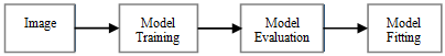
Active Shape Model (ASM) is a flexible segmentation methodology (see Figure 1) that has been used for segmentation of a wide range of images such as medical images and facial images [1-3]. The Information used in the ASM consists of mainly shape and its intensity. The shape of an object is defined as interconnected sets of landmark points. The shape intensity is the set of all the intensities that describe the local appearance of its landmarks points. Formally, ASM is structured around three main components: 1-A Statistical Shape Model, 2-A set of Local Appearance Models and 3-A matching procedure. The shape model describes the shape variability of a set of deformable objects. The local appearance models describe the intensity variability around each landmark. The matching procedure consists of fitting the shape model to an object in order to localize its shape. The local features of a landmark are used as criteria to guide the detection process of points during the matching procedure. The success of the ASM model lies in its ability to find the right positions of all landmark points which define the object shape.
Figure 1. Stages of model-based segmentation
The first local appearance models used in ASM were the normalized first derivatives of perpendicular profiles at the shape and centered at each landmark. The matching procedure consisted therefore of finding the strongest edge along the profile of each land-mark. However, the approach seems to fit only to simple situations, but in most real problems it might fail and generate false positions (i.e. noisy observations). Therefore, locating landmarks is a critical operation in the matching procedure that greatly affects the performance of the segmentation. In recent years, several segmentation approaches based on ASM have been found in the literature in order to improve the ASM performance. This paper concentrate on intensity models proposed in the literature for the ASM model, in order to give a review and a discussion about their method and their impact on the segmentation performance.
The remainder of the paper is organized as follows: In section 2, we describe the ASM standard method. In section 3, we define the common framework of process of establishing of the local appearance models, and we formulate in a combined way the principle of the matching procedure using these models. In section 4, we review the different intensity models given in the literature. We discuss these models in section 5. Finally, conclusions and perspectives are given at the end.
Model-based methods make use of a prior model of what is expected in the image and try to find the best match of model to the data in a new image. The first works described by Cootes et al. showed how to construct the models of a set of deformable objects, called Point Distribution Models (PDM), and how to use them to adapt them to the image [1, 2]. In this section we briefly describe the ASM model and its formal framework, as well as the matching procedure principle.
2.1 Statistical Shape Models
Statistical Shape Models are PDM which represent the shapes according to their main modes of variation independently of their poses in the reference of the image. For any set of model parameters, one can generate an instance of the model and project it into the image frame. Thereby, fitting a PDM model to a new image means find the model parameters that define both the shape and position of the target object.
Given a set of training images for a given object, each object shape is represented by a sequence of n points placed in the same location on the object in each image. The set of points forms a shape vector X such as:
$X=\left\{\left(x_{i}, y_{i}\right)\right\} i=\overline{1, n}$ (1)
If we have N training examples, we generate N shape vectors $X_{j}$. The average shape $\bar{X}$ of the training set is calculated from an iterative procedure such that all the shapes $X_{j}$ are aligned to the tangent space of the $\bar{X}$.
$\bar{X}=\frac{1}{N} \sum_{j=1}^{N} X_{j}$ (2)
Lastly, Principal Component Analysis (PCA) is applied to the set of the aligned vectors $X_{j}$. These vectors $X_{j}$ form a cloud of points in a 2n dimensional space. PCA method is applied to reduce the dimensionality of the data from 2n to something more manageable, by determining the major axes of points cloud. Each axis gives a mode of variation, a way in which the landmark points tend to move together as the shape varies. The approach is summarized as follows:
(1) For each vector Xj, we compute its deviation dXj from the average shape $\bar{X}$:
$d X_{j}=\left|X_{j}-\bar{X}\right|$ (3)
(2) We compute the shape covariance matrix S:
$S=\frac{1}{N} \sum_{j=1}^{N} d X_{j} d X_{j}^{T}$ (4)
(3) We compute the eigenvectors $\{\varphi\}$ corresponding to the largest eigenvalues l such as:
S. $\varphi=\lambda . S$ (5)
Any shape X (See Eq. (1)) can be approximated by the nearest point (See Eq. (6) in the new space $\{\varphi\}$ of origin $\bar{X}$. A point in this subspace (See Eq. (7)) is defined by a vector b of shape parameters.
$X=\bar{X}+\varphi . b$ (6)
$b=\varphi^{T}(X-\bar{X})$ (7)
By varying b, one can vary the shape X using Eq. (6). The variance of b, across the training set is given by l. By applying limits of $\pm 3 \sqrt{\lambda}$ to the parameter b, one ensures that the shape generated is similar to those in the original training set.
2.2 ASM matching
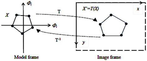
Figure 2. Bijection (T) between image frame and model frame
Matching procedure is defined as an iterative approach that allows a reliable comparison between the PDM model and an object of interest in an image. It is based on the change of reference between the image frame and that of the model (See Figure 2), in order to calculate the best pose and model parameters of the target object. In theory, the matching corresponds to an optimization problem of a parameterized fit function between a model instance and image.
Given Xb an instance of model and its variant Xb,pof pose p, and an object Y, the formulation of the principle of the ASM matching is as follows:
Find b and p which optimizes:
$F_{b, p}=\left|Y-X_{b, p}\right|$ (8)
Under the constraints:
$X_{b}=\bar{X}+\varphi . b$ (9)
$X_{b, p}=(\bar{X}+\varphi . b)_{p}$ (10)
This formulation (See Eqns. (8-10)) depends essentially on the choice of the fit function F, the model X and the object Y, whatever the optimization method used to find the optimum. It is the fundamental principle of ASM method whose goal is both to seek a set of shape parameters and improve the fit of X to Y. In principle, the problematic of the ASM method is the same in any dimensions.
In practice, the matching procedure consists of finding all the possible and correct adjustments between the model and the object in order to identify its landmarks and delimit its outline. The standard matching algorithm uses the average shape model to approximately express the shape of target and then matches it to the target object by limiting the variable shape parameters. The basic assumption is that usually the desired landmarks points are located on the strong edges that correspond to points whose intensity gradients are maximized. Precise and strong location of shape points is a complicated and difficult issue in object localization. Improved matching algorithms based on the traditional ASM matching were proposed in the literature. Some works propose to modify the practice of the matching procedure and others propose to speed it up in order to increase its performance. Liao and Wu [4] propose a shape evaluation method and a weighted matching procedure using the evaluation information. Zhao et al. [5] add a process of searching the most similar image to the target object from the training sample set and uses the shape model of the similar image instead of the average shape model to approximately express target object model. Wang et al. [6] evoke the fine grain parallelism and applies it to the matching algorithm and reformulate it as a parallelizable algorithm. The parallel version of matching algorithm is implemented in a multi-core (CPU/GPU) environment. Naoui et al. [7] propose a theoretical framework to implement a distributed and parallel version of ASM and AAM methods.
In order to reinforce the matching procedure, ASM method broadens its modeling by integrating the modeling of the local appearance of shape landmarks. The description of any object is thus established from a combination of an explicit shape model and a set of local appearance models. The idea is to use them to locate new landmarks and correct their locations if necessary by looking at how these new landmarks are located with respect to each other. In this section, we present the common framework of building local appearance models in the ASM and then we reformulate the principle of the matching procedure described in the previous section, taking into account both the shape model and the appearance local models.
3.1 Principe of building
A local appearance model of a shape landmark point is commonly established by an intensity model which captures the features of interest of landmark and allows a reliable comparison during matching procedure. It is generated during the modeling phase of the ASM and is used in the process of detecting new points during the matching procedure.
Let an intensity model [8] composed of a feature extraction function f and a similarity measure h. Let S be a set of N shapes $X_{i}$ each composed of n points labeled Aij, patches Pij of pixels centered at each point Aij are extracted from each shape $X_{i}$, building the following set:
$\forall X_{i} \in \mathrm{S}, D_{i}=\left\{P_{i j} / \overline{J=1, n}\right\}$ (11)
The extractor f applied in each patch Pij, consists in extracting a set of local features fij that describes the local texture around each landmark Aij for all the training images, such as:
$\forall i=\overline{1, N}, \forall j=\overline{1, n}, f_{i j}=f\left(P_{i j}\right)$ (12)
An average of features $\bar{f_J}$ for each landmark Aij can be computed as follows:
$\forall j=\overline{1, n}, \bar{f_J}=(1 / N) \sum_{i=1}^{i=N} f\left(P_{i j}\right)$ (13)
A separate template Tj of local features can be generated for each landmark Aij as follows:
$\forall j=\overline{1, n}, T_{j}=M\left(\left\{f_{i j}\right\}\right) \overline{\imath=1, N}$ (14)
M is a model generation function defined in the modeling phase of the ASM and applied to all features of the point j in all images. The similarity measure h is used to compute the difference of similarity between the features of two shape points, whose one is generated by the template T and the other, is generated by the extractor f, such as:
$k, j \in X / D=h\left(T_{j}, f_{k}\right)$ (15)
It is used as criterion of local search to detect in a restricted area the points that match each other. In other terms, it is used to find the point k among the points of a region Rj, closest to point j in terms of characteristics such as:
$\forall j \in X$ Find $k \in R_{j}$ such as $f_{k} \cong T_{j}$ (16)
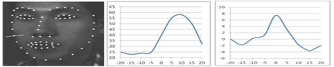
An example of such model is 1D-profile (as shown in Figure 3) of the original version of the ASM [2, 3]. The extraction function f corresponds to the sampling of the intensity or even its gradient along the normal to the landmark point. The generation model M is the method PCA used to generate the templates T. The similarity measure h corresponds to the calculation of the Mahalanobis distance between a search profile and the template of each landmark point.
Figure 3. (a): landmarks and a normal vector direction at a specific landmark point, (b): intensity profile, and (c): gradient profile
3.2 Expanded matching procedure
Matching procedure in ASM method is based principally on the use of PDM model in the search of the shape of an object, as described in the preceding section. Transformations operate on the shape model to fit it to the test image. Iterative processing is performed on the shape in order to find suitable final landmarks. These landmarks will form a shape that best suits the test image. In order to achieve this end, the use of the local appearance models in matching procedure is an approach adopted to find the better locations of landmarks and conceive a new shape. Best locations of the landmarks are determined through a two-step search process:
(1) Establishing the profiles of the points neighboring the landmark,
(2) Selecting the point whose profile is closest to the landmark appearance model (See Eq. (16)).
This process is repeated for each landmark before handing control back to the shape model. The profile of a point, called search profile, is determined by the features extraction function as that applied during building the local appearance model of a landmark point (See Eq. (12)). The principle of the ASM method is thus to alternate the PDM model and the local appearance models iteratively until locate the target object shape. We thus rewrite the principle of matching described in paragraph 2.2 (See Eqns. (8-10)), by integrate the profile of shape points, determined by the two-step search process outlined above.
The matching goal is therefore to determine the parameters of model b, of pose p and of appearance c, which best the model to the image and thus make it possible to locate the target object Y. The formulation of ASM method becomes:
Find b, p and c which optimizes:
$F_{b, p ; c}=\left|Y-X_{b p c}\right|$ (17)
Under the constraints:
$X_{b p c}=\left(X_{b p}, c\right)$ (18)
$X_{b p}=(\bar{X}+\varphi \cdot b)_{p}$ (19)
$c=\left\{g_{y} / y \in X_{b p}\right\}$ (20)
Such as:
$\forall y \in X_{b p}, g_{y}$ is the best matching of $T_{y}$ (21)
Tx is the model of the local appearance of point y. gy is the profile of point better y established according to the two-step search process in the space of the image. Xbp represent the set of the better points y of appearance gy. Xbp takes the form of estimates for the position at which the instance model should be placed, and for the orientation, scale and shape parameters required to fit it to the image. Xbp is thus the new shape to be converted into an appropriate shape and to be improved to represent the shape of the target object Y.
All the propositions are correlated with each other and it is difficult to find until now a formal approach that calculates the possible adjustments to be used to delimit the outline of the target object in the image space. Finding the correct adjustments is thus both crucial and difficult step of the ASM method.
One finds in the literature several ways to modify, refine, and improve the different components of ASM. Some works adopted the ASM original version and they adapted it to their applications, while others proposed to use the ASM strategy with modifications. In this section, we cite the proposals that have specifically addressed the issue of intensity models for local description of the image features and features detection. Tables 1 and 2 summarize the intensity models, the profile template, the similarity measure and the image type.
4.1 ASM intensity models
As mentioned earlier, the first model of local appearance established in the ASM method is the 1D-profile. In the improved version, Cootes et al. proposed to use the normalized first derivatives of the profiles to build the 1D-Gradient-profile, commonly called 1D-profile [1, 2]. Gradients are used because they are invariant to the overall light level and their normalization helps make the profile invariant to changes of overall contrast at the landmark. Each profile model is represented by the mean and the covariance matrix of the set of profiles of fixed-length extracted for each point during modeling stage. During the search, the point whose the profile satisfies the criterion of least distance of Ma-halanobis is assumed to be the most likely landmark location. In order to fast convergence, a multi-resolution strategy is adopted.
Table 1. ASM-intensity models, profile template, similarity measure and images type
|
Paper |
Intensity Model |
Profile Template |
Similarity Measure |
Images |
|
Cootes et al. [2, 3] |
ASM 1D-profile |
Covariance Matrices |
Mahalanobis distance |
Medical, face |
|
Mahoor et al. [9] |
ASM 1D-profile |
Multivariante Gaussian Models |
Weighted sum of Mahalanobis distances |
Public color images |
|
Josephson et al. [10], Tobon-Gomez et al. [11] |
ASM 3D-profile |
Mean profiles |
Mahalanobis distance |
3D-medical (brain,cardiac) |
|
Critinacce et al. [6] |
AAM local texture |
Mean, Covariance matrices |
CLM search |
Face |
|
Iqtait et al. [13] |
AAM global texture |
Mean, Covariance matrices |
Non Linear Gradient Descent |
Face |
|
Seghers et al. [14] |
ASM spherical 2D-profile |
Mean, Covariance Matrices |
Intensity cost of Mahalanobis distances |
3D-Medical (liver CT) |
|
Nanayakarra et al. [15] |
ASM Morphologic 1D-profile |
Mean, Covariance Matrices |
Mahalanobis distance |
Breast skin line (mammogram) |
|
Labrunie et al. [16] |
ASM 1D-profile |
Profile Classes using k-means algorithm |
Mahalanobis distance |
Medical (Orofacial articulators) |
|
Lee et al. [17] |
ASM square 2D-profile |
Average |
Difference of profiles |
Face |
|
Seghers et al. [18] |
Gibbs function of Probability distribution functions of the intensities |
Covariance Matrix (Gaussian Distribution) |
Mahalanobis distance |
3D-Medical (hand bone, liver) |
Table 2. Modified intensity models, profile template, similarity measure and images type
|
Paper |
Intensity Model |
Profile Template |
Similarity Measure |
Images |
|
Ginneken et al. [19] |
Multiscale Gaussians derivatives |
First and second moments of local histogram |
KNN-classifier |
Medical (lung) |
|
Li et al. [20] |
Steerable filters |
Adaboost |
AdaBoost classifier |
Medical (brain) images |
|
Cootes et al. [21], Lindner et al. [22] |
Haar wavelets |
Histogram of vote (HOV) |
Random Forest Regression Voting |
Medical (hand), face |
|
Ebhotemhen et al. [23] |
Haar filters |
KNN machine learning |
KNN classifier |
Brain |
|
Le and Vo [24] |
2D-Sobel filter |
SVM machine learning |
SVM classifier |
Public faces |
|
Huang et al. [25] |
2D-Gabor filter |
Gabor kernels |
Phase-Sensitive Similarity Function and Beier-Neely algorithm |
Faces (Jaffe, Yale) |
|
Spinczyk et al. [26] |
1D-profile |
Gaussian distribution |
Mahalanobis distance |
Medical (liver) |
|
Zhou et al. [27] |
Local SIFT and ASM 1D-profile |
Local gradient direction histograms, Covariance m |
Nearest neighbors, Mahalanobis distances |
Face |
|
Zhou et al. [28] |
POEM |
Mean of POEM histograms |
Chi-square distance |
Face |
|
Milborrow et al. [29, 30] |
HAT |
Regression model: Decision trees |
Multivariate Adaptive Regression Splines |
Face |
|
Antonakos et al. [31] |
HOG, SIFT, LBP |
AAM covariance Matrices |
Gradient descent Inverse Compositional |
Face |
|
Medley et al. [8] |
Local texture |
ASM-FTT, ASM-VTT: Covariance |
Cross-correlation between templates |
Medical (left ventricle), Face |
Several works have adopted the original ASM and they adapted it to their applications.
For example, for color images, 1D-profile is computed in each component of color space. Mahoor et al. [9] devised an approach using a weighted sum of three multivariate Gaussian models for the three components of RGB (Red, Green, and Blue) color space to conceive the 1D-profil. They used a weighted sum of the three Ma-halanobis’s distances corresponding to the three channels of RGB color space as a criterion, in order to find the best matching. They validate their approach by experimenting a database composed of different subjects provided from different sources and other public databases. The approach seems to be partially automated.
For multidimensional images, Josephson et al. [10] have developed a fully automated segmentation system of the medical images in three-dimensional using ASM. 1D-gradient profile along a perpendicular at each surface is built for each landmark. During profile matching, edge detection is performed on a short distance along the normal to the surface to find the new positions of each landmark. The best positions are determined using Mahalanobis distance. The method was experimented on Magnetic Resonance (MR) images of the knee and SPECT images of the brain, without any indication on the implementation of the proposed method. The authors validated their approach that depends strongly on the quality of initial guess.
Tobon-Gomez et al. [11] proposed to build a 3D-intensity model composed of 1D- profiles directly given from real medical (cardiac) images, using medical imaging simulators. A 1D-profile is calculated for each endocardial and epicardial wall by sampling the gradient of the profile intensities along a perpendicular to each mesh of cardiac image. During matching, new positions are obtained by selecting the minimal Mahalanobis distance between sampled profiles and mean profiles of the intensity model. The proposed method was tested on two datasets, one for an automated build of 3D-intensity models and the other for evaluation of their performance. Simulation software was used to generate structures for study. Simulations were run using a computing grid of a cluster of 20 dual-processors. The feasibility of the approach was confirmed for cardiac images. However, the approach was considered difficult to manage, and many parameters were hard to determine.
Although the 1D-profile is a key method that works as well as any, it is also a sensitive technique in some situations. To Base solely on intensity gradients and searching along a perpendicular direction, can cause mapping errors during search process that misguide the estimation of the ASM parameters. In this case, the accuracy of the ASM is severely compromised, resulting in a decreased segmentation performance. Complementary approaches have been proposed to overcome the ASM drawback such as the AAM model [3] and later the CLM model (Constrained Local Model) [12] which is similar to AAM in the sense that it applies the AAM formalism inside a small area surrounding the landmark point. In the same context, Iqtait et al. [13] proposed to use jointly the ASM model and AAM model, and test their performance on one dataset of faces. ASM and AAM are presented in their standard version. One hundred (100) face images are chosen as training set, each marked with 68 points. The experiments conducted show that the number of searching positions has the most primary influence on the location result. They compared the performance between both algorithms with respect to point to point errors and execution time measurements. They conclude that the ASM algorithm locates the points more accurately and faster than the AAM algorithm. The experiments were conducted on Matlab environment without specifying the detail of the implementation.
Although ASM and its complementary approach have contributed a lot to the field of object detection, there are still shortages on real world problems. Other works adopted the ASM strategy but slightly modified in order to compensate the deficiency in the ASM search process.
Seghers et al. [14] proposed to use a spherical intensity profile collected on a sphere centered at each landmark in a 3D image. A statistical intensity model similar to 1D-profile of a 2D image is obtained by estimating the mean and the covariance of features of each landmark point. The similarity function called intensity cost is computed in 3D, similar to that of 2D of ASM. In the search process, a grid is defined around each model point to extract a set of candidate locations. For each candidate point, a search function is computed taking account both initial cost function and shape knowledge. The best candidate is selected if its search function is optimal. The search process was done in a multi-resolution framework. The proposed method was tested and validated for the liver CT (Computed Tomography) images in contrast enhanced. The different operations of the proposed approach have been implemented in Matlab. The approach has consumed a considerable calculation time estimated at twenty minutes.
Nanayakarra et al. [15] developed an automatic segmentation method of breast skin line. They have used intensity gradient information to initial boundary estimation, and morphologic operators to final boundary estimation of breast images. An 1D-gradient profile is used to extract the boundary points and estimate end points on the skin line. The method was tested and validated on many mammograms taken from a mini popular database among mammogram research community.
Labrunie et al. [16] introduced a method for predicting mid-sagittal contours of orofacial articulators from real time MR (Magnetic Resonance) images, using ASM slightly modified. A 1D-profile similar to that of original ASM is built for each point of each articulator at two resolution levels of image. The intensity profile is sampled by interpolation on the points distributed along a normal segment by step of one pixel. The obtained intensity profiles are then categorized in two classes “Contact and No contact”. These classes serve to measure and test the distance between the contour points to the nearby articulators. Each class is divided by a k-means algorithm into subclasses. Each subclass is represented by its average profile. The distances of all profiles at the average profiles were calculated. The classes serve then to determine the new positions of landmark points. The approach was evaluated from a corpus of about 26 minutes of speech of a French speaker at a rate of 55 MR images /s. The efficiency of the presented method was demonstrated by the authors.
Lee et al. [17] presented a method of extraction of facial point features that operates on mobile devices. They proposed to extend 1D-profile to a 2D-profile model. A square region is selected for each landmark. The average of gray-levels of each point within the square is computed. To locate the new locations of each model point, they proposed a similarity function based on the calculation of the difference of two profile matrices. The first matrix represents 2D-profile of a model point and the second matrix represents its sub 2D-profile. The method was implemented using Java and C with Eclipse via the android platform. It was validated on various images from JAFFE dataset, Google search and their own faces. The results obtained showed slightly higher efficiencies in terms of computational time compared to the original version of ASM.
Seghers et al. [18] presented an intensity model constructed by estimating the probability distribution functions of the intensity patterns in an image around each landmark. Thus, Gibbs function is estimated for each landmark individually. The set of intensity models is modeled as a Gaussian distribution. The Mahalanobis distance is used for the intensity models matching. The approach has been validated using hand bone and 3D liver images.
4.2 Modified ASM intensity models
Several works tried to choose better local appearance models completely different from the 1D-Gradient profile, in order to achieve high segmentation accuracy. Some works are inspired by the research work, particularly in the field of artificial intelligence and pattern recognition. Other works have resorted to the use of some robust image matching techniques known in the field of machine vision and robotics.
For example, Van Ginneken et al. [19] proposed both an intensity model composed of optimal local features along a perpendicular to the object contour instead of the normalized derivatives of 1D-profile, and a nonlinear classifier instead of the Mahalanobis distance. Multi-scale Gaussians derivatives of images are computed to describe local image structure. Around each landmark, the first and second moments of a local histogram are extracted. At each resolution, a square region is thus defined in order to extract a features vector. The optimal features are determined by using a selection technique of features and a nonlinear classifier of the k-Nearest Neighbors (KNN- classifier). During search, a considerable set of features along a normal profile is computed and fed to classifier in order to determine if the point is inside or outside the object. The method was experimented by using different types of data, in particular lung images, in order to show the course of all operations and measure the method performance. The method does not seem to be completely automated and, the implementation and its environment are not described.
Li et al. [20] have used steerable filters to extract local edge orientation features. A structure cantered at each landmark is defined by a square grid. For each grid point, a set of features is extracted varying parameters of steerable filters. The structure of local edge at each landmark is thus described by the set of features of all points of the grid. A machine learning algorithm based on AdaBoost algorithm is introduced to construct a classifier for each landmark. During search process, the classifier serves to determine the next move of the landmark point by analyzing its features along the perpendicular to the shape contour, if it is edge or non-edge. The approach was tested on brain images in which the corpus callosum was labelled manually. The approach was validated by comparing the final positions of model points to their correspondents manually labelled, by calculating the distance between them. The approach is not fully automated. The implementation in Matlab is partially described. The training process is off-line. The feature images and the classification have been done on-line. The approach used have consumed more time than the original version of ASM.
Cootes et al. [21] and later Lindner et al. [22] used the Random Forest Regression Voting approach to generate the optimal positions and locating new shape points during search process. For each landmark, a set of features of neighbouring points taken at a random distance is determined. A voting approach is thus applied in a grid over the region of interest to predict the most likely positions to the landmark point, and select thus the best position. A histogram of vote (HOV) is established to define the landmark descriptor. During search, each descriptor predicts one or more positions of the target point. Votes are accumulated in a grid to then select the best position for the landmark. The approach was validated on a range of datasets, face images and medical images.
Ebhotemhen [23] proposed to use the K-Nearest Neighbor (KNN) machine learning in the process of segmentation of medical images in order to improve segmentation accuracy. Haar filters are used as intensity model to extract features of landmarks. KNN is used to learn better positions for each landmark and to classify points around the final points of the search process of ASM. The author validates his approach by processing a set of 86 brain images annotated with 15 points each, showing that machine learning can be used to improve automatic segmentation accuracy of medical images.
Le and Vo [24] suggested to use a model combining Sobel filter and the 2D-profile in the local search process of ASM. Support Vector Machine (SVM) is used to classify and determine the new positions of landmarks. The proposed method was tested and validated on public face images from Denmark databases.
Huang and Hsu [25] proposed a facial feature location method based on active shape model and Gabor filter to reduce the intensity contrast and to enhance edge information. They use firstly 2D Gabor filter to extract the facial features and then to use a square region in the search process to decrease the location error. To locate the facial features, they proposed to use both the Gabor kernels reduction and local feature-based weighted warping method. They tested their approach using JAFFE and Yale [21] face databases under various viewing conditions of pose and illumination. To estimate the performance of their approach, a manual labeling and Viola-Jones face detector were utilized. The results obtained show that their approach is moderately robust to illumination variation. The approach seems not to be completely automated.
Spinczyk and Krasoń [26] authors proposed an automatic liver segmentation using general purpose shape modeling methods. The atlas based segmentation was used as being the simplest shape-based method. Subsequently, the ASM method was applied with optimal features as defined in the study [14]. Lastly, a generalization of classical statistical shape models, the Gaussian Process Morphable Models (GPMM), was used. The preferred method is that of GPMM which is based on the multi-dimensional Gaussian distributions of the shape deformation field. The GPMM are used as a process of generation of candidate points for the location of the model points during search process. The new locations result from the probability distribution of the shape deformation field. Mutual information and sum of square distance were used as similarity measures. 20 CT images of the abdominal cavity were used for the liver segmentation. The obtained results are compared to that dedicated for liver segmentation. The dice similarity was used as a statistical validation metric to evaluate the performance of the used methods. The best results were obtained for the GPMM method.
Zhou et al. [27] proposed to use SIFT (Scale Invariant Feature Transform) descriptors and the gray-level profiles for an automatic search of the landmarks in the face images. A Human face has been represented both by SIFT descriptor and a 1D-gradient profile. Different face data have been used for experiments, using the face detector of Viola-Jones and the STASM software. The proposed approach has shown an increased performance than the standard approach of ASM but worse than the STASM software.
Zhou et al. [28] proposed to use the Patterns of Oriented Edge Magnitudes (POEM) descriptor to represent the local appearances of the landmarks instead of pixel intensity values. A gradient image is firstly computed to determine the magnitudes matrix and directions matrix. For each pixel, a features vector is then computed composed of its magnitude and a set of magnitudes of region surrounding it. Similarity function is thus the difference of gradient magnitudes. A square region cantered at each landmark is then considered to compute finally its local appearance pattern. A set of POEM histograms is thus computed. The average histogram of each landmark acts as a local appearance model. The computing of similarity between histograms is determined using the Chi square distance. The approach was validated by using a considerable set of face images under various poses and illuminations. The implementation of the approach is not described and the approach but seems also not to be completely automated.
Milborrow et al. proposed a Histogram Array Transform (HAT) descriptor which is a simplified form of SIFT descriptor [29, 30]. HAT descriptor is unrotated SIFT descriptor with a fixed scale. Decision trees are used to generate the model for a landmark that predicts goodness-of-fit as a function of the elements of the descriptor. A Multivariate Adaptive Regression Splines (MARS) is used for descriptor matching. The descriptor has been implemented using OpenCV (Open Computer Vision) and OpenMP (Open Multi-Processing) to reduce its computational load. The approach has been experimented on facial images for validating.
Antonakos et al. [31] proposed to use the dense appearance features images for both Lucas-Kanade alignment algorithm and AAM fitting algorithm. Several descriptors have been used to extract image features mainly Histogram of Oriented Gradients (HOG), SIFT and Local Binary Patterns (LBP). Extracting features from image and warping improves significantly the approach performance and decreases its computational complexity. The optimization technique used is the gradient descent Inverse Compositional. The approach was tested on a set of face images downloaded from the web captured in totally unconstrained conditions. The presented experiments prove that HOG and SIFT are the most powerful descriptors. The implementation of the proposed approach is not described.
Medley et al. [8] proposed a methodology composed of two detection methods of the reliable observations points called ASM-FTT (ASM-Fixed Texture Templates) and ASM-VTT (ASM-Variable Texture Templates) that are used in the ASM framework. The two approaches use a rectangular region sampled around each landmark point conforming to a features template defined over training set. In ASM-FTT, the template is fixed and it is characterized by a mean texture of the region surrounding each landmark point. In ASM-VTT, the template is formulated as the CLM model [12]. It is variable and it is characterized by a linear combination of main variation modes obtained by the PCA (Principal Component Analysis) analysis of local texture surrounding each landmark point. During search process, the same templates are used to define a search region which is compared to the templates via a specific correlation function. The methodology was applied to facial images and medical images. The authors have compared the performance of their methodology against three detectors based on classical ASM edge detector, HOG detector and SIFT detector. The obtained results show that the proposed approach is better than the other three approaches. The implementation of the proposed approach is not described.
Reviewing works described in section 4, the feature detection and image matching form the core of the segmentation approach directed by the ASM model. Many intensity models have been proposed as part of the ASM to better frame the issue of the location of shape points during the matching procedure. Each intensity model is defined by the nature of its features, and its similarity function. The majority of intensity models used two-dimensional or three-dimensional images.
In the category of ASM models, 1D-profile is often used to create the multidimensional profiles, the nD-profiles (n>1). Intuitively, the nD-profile can obtain more information around the landmark which can also offer a better result on model fitting. The transition to an nD-profile is proposed in different ways. The distance of Mahalanobis is used in the most of search methods.
The models completely different from 1D-profile propose other strategies in terms features and search. Applying powerful local features extractors, broadening the area of search, anticipate good research directions constitute the core of such intensity models, whose aim is to compensate the deficiency in the search process of the 1D-profile and improve active shape model segmentation. The machine learning based classification and regression methods are the new proposals applied in the search process.
The performance of proposed intensity models is strongly influenced by several factors such as accuracy, invariance, and ability to deal with the complex shapes. If the accuracy and robustness characterize at a level considered satisfactory the new descriptors, the efficiency parameter is hard to achieve. The robust intensity models are considerably more expensive in computing time than of original ASM. They require a large computational complexity to increase accuracy and robustness. The abundance of features leads to more time in searching for the right profiles. The classification and regression methods improve the quality in terms of accuracy and robustness of matching but require the characteristic of non-linearity of some descriptors which also brings in great computational complexity [32].
The price to pay to increase accuracy and robustness is thus that of a higher computational load which can be a major drawback especially for real-time applications. The computational load is clearly concentrated at image description and on comparison between profiles.
Implement these intensity models, reduce their computational complexity under specific conditions, such as in real time systems, and make them applicable to practical real-world applications are again a challenge for ASM-related community [7, 33-35].
In this paper, we attempted to provide a comprehensive overview of several researches on intensity models proposed in the literature as the alternatives to ASM 1D-profile. For this purpose, the formal framework of intensity model is described, followed by an expanded formulation of the ASM matching including profile matching. We have taken a deep survey for understanding the proposed methods. The various proposals along with their advantages and disadvantages are discussed in this paper. The studies presented in this paper provide a basis for conducting our project future in this area.
|
A |
shape point |
|
b |
shape parameter vector |
|
c |
set of profiles |
|
D |
set of patches |
|
F |
Fit function |
|
f |
feature extraction function |
|
g |
profile of point |
|
h |
similarity measure |
|
M |
model generation function |
|
N |
number of examples |
|
P |
set of pixels |
|
p |
shape pose |
|
R |
region of point |
|
S |
set of shapes |
|
T |
template of local feature of point |
|
X |
shape vector |
|
$\overline{\mathrm{X}}$ |
shape average |
|
Y |
object |
|
Greek symbols |
|
|
$\lambda$ |
eigenvalue |
|
$\varphi$ |
eigenvectors |
|
Subscripts |
|
|
b |
shape parameter |
|
c |
shape appearance |
|
i |
index |
|
j |
index |
|
k |
shape point |
|
p |
shape pose |
|
y |
shape point |
[1] Cootes, T.F., Taylor, C.J., Cooper, D.H., Graham, J. (1995). Active shape models - their training and applications. Computer Vision and Image Understanding, 61(1): 38-59.
[2] Cootes, T.F., Taylor, C.J. (1997). A mixture model for representing shape variation. Image and Vision Computing, 17(8): 567-574. https://doi.org/10.1016/S0262-8856(98)00175-9
[3] Cootes, T.F., Edwards, G.J., Taylor, C.J. (1998). Active appearance models. European Conference on Computer Vision, pp. 484-498. https://doi.org/10.1007/BFb0054760
[4] Liao, C., Wu, X. (2013). An improved ASM matching method. Proceedings of the 2nd International Conference on Computer Science and Electronics Engineering, pp. 1773-1776. https://doi.org/10.2991/iccsee.2013.444
[5] Zhao, M., Li, S., Chen, C., Bu, J. (2004). Shape evaluation for weighted active shape models. Proceeding of the Asian Conference on Computer Science.
[6] Wang, J., Ma, X., Zhu, Y., Sun, J. (2014). Efficient parallel implementation of active appearance model fitting algorithm on GPU. The Scientific Word Journal, 528080. https://doi.org/10.1155/2014/528080
[7] Naoui, M., Mahmoudi, S., Belalem, G. (2016). Feasibility study of a distributed and parallel environment for implementing the standard version of aam model. Journal of Information Processing Systems. 12(1): 149-168. https://doi.org/10.3745/JIPS.02.0039
[8] Medley, D., Santiago, C., Nascimento, J.C. (2018). Robust feature descriptors for object segmentation using active shape models. International Conference on Advanced Concepts for Intelligent Vision Systems, pp. 163-174. https://doi.org/10.1007/978-3-030-01449-0_14
[9] Mahoor, M.H., Abdel-Mottaleb, M., Ansari, A.N. (2006). Improved active shape model for facial feature extraction in color images. Journal of Multimedia, 1(4): 21-28. https://doi.org/10.4304/jmm.1.4.21-28
[10] Josephson, K.., Ericsson, A., Karlsson, J. (2005). Segmentation of medical image using three-dimensional active shape models. Scandinavian Conference on Image Analysis, pp. 719-728. https://doi.org/10.1007/11499145_73
[11] Tobon-Gomez, C., Butakoff, C., Aguade, S., Sukno, F., Moragas, G., Frangi, A. (2008). Automatic construction of 3D- ASM intensity models by simulating image acquisition: Application to myocardial gated SPECT studies. IEEE Transactions on Medical Imaging, 27(11): 1655-1667. https://doi.org/10.1109/TMI.2008.2004819
[12] Cristinacce, D., Cootes, T.F. (2006). Feature detection and tracking with constrained local models. Proceedings of the British Machine Conference, pp. 1-10. https://doi.org/10.5244/C.20.95
[13] Iqtait, M., Mohamad, F.S., Mamat, M. (2018). Feature extraction for face recognition via active shape model (ASM) and active appearance model (AAM). IOP Conference Series: Materials Science and Engineering, 332(1): 012032. https://doi.org/10.1088/1757-899X/332/1/012032
[14] Seghers, D., Slagmolen, P., Lambelin, Y., Loeckx, J.D., Maes, F., Suetens, P. (2007). Landmark based liver segmentation using local shape and local intensity models. Proc. Workshop of the 10th Int. Conf. on MICCAI, Workshop on 3D Segmentation in the Clinic: A Grand Challenge, pp. 135-142.
[15] Nanayakarra, R.R., Yapa, Y.P.R.D., Hevawithana, P.B., Wijekoon, P. (2015). Automatic breast boundary segmentation of mammograms. International Journal of Soft Computing and Engineering (IJSCE), 5(1).
[16] Labrunie, M., Badin, P., Voit, D., Joseph, A.A., Lamalle, L., Vilain, C., Boë, L., Frahm, J. (2016). Tracking contours of orofacial articulators from real time MRI speech. 17th annual Conference of the International Speech Communication Association, San Francisco United States, pp. 470-474. https://doi.org/10.21437/Interspeech.2016-78
[17] Lee, Y.H., Yang, D.S., Park, Je., Kim, Y. (2013). Facial feature extraction using enhanced active shape model. 2013 International Conference on Information Science and Applications (ICISA), Suwon, pp. 1-2. https://doi.org/10.1109/ICISA.2013.6579397
[18] Seghers, D., Hermans, J., Loeckx, D., Maes, F., Vandermeulen, D., Suetens, P. (2008). Model based segmentation using graph representations. International Conference on Medical Image Computing and Computer-Assisted Intervention, pp. 393-400. https://doi.org/10.1007/978-3-540-85988-8_47
[19] Van Ginneken, B., Frangi, A.F., Staal, J.J., ter Haar Romeny, B.M., Viergever, M.A. (2001). A non-linear gray-level appearance model improves active shape model segmentation. Proceedings IEEE Workshop on Mathematical Methods in Biomedical Image Analysis (MMBIA 2001), Kauai, HI, USA, pp. 205-212. https://doi.org/10.1109/MMBIA.2001.991735
[20] Li, S., Zhu, L., Jiang, T. (2004). Active shape model segmentation using local edge structures and adaboost. International Workshop on Medical Imaging and Virtual Reality, 121-128. https://doi.org/10.1007/978-3-540-28626-4_15
[21] Cootes, T.F., Ionita, M.C., Lindner, C., Sauer, P. (2012). Robust and accurate shape model fitting using random forest regression voting. European Conference on Computer Vision, pp. 278-291. https://doi.org/10.1007/978-3-642-33786-4_21
[22] Lindner, C., Bromiley, P.A., Ionita, M.C., Cootes, T.F. (2014). Robust and accurate shape model matching using random forest regression-voting. IEEE Transactions on Pattern Analysis and Machine Intelligence, 37(9): 1862-1874. https://doi.org/10.1109/TPAMI.2014.2382106
[23] Ebhotemhen, E. (2013). Medical image segmentation using an extended active shape model. International Journal of Computer Applications, 69(19): 0975-8887.
[24] Le, T.H., Vo, T.N. (2012). Face alignment using active shape model and support vector machine. arXiv preprint arXiv:1209.6151.
[25] Huang, H., Hsu, S. (2011). Improved active shape model for facial feature localization. IEEE Transactions on Medical Imaging, 21(8).
[26] Spinczyk, D., Krasoń, A. (2018). Automatic liver segmentation in computed tomography using general-purpose shape modeling methods. Biomedical Engineering Online, 17(1): 65. https://doi.org/10.1186/s12938‑018‑0504‑6
[27] Zhou, D., Petrovska-Delacretaz, D., Dorizzi, B. (2009). Automatic landmark location with a combined active shape model. 2009 IEEE 3rd International Conference on Biometrics: Theory, Applications, and Systems, Washington, DC, pp. 1-7. https://doi.org/10.1109/BTAS.2009.5339037
[28] Zhou, L., Fang, B., Li, W., Lai, P. (2013). Improved active shape model for facial feature localization using POEM descriptor. 2013 International Conference on Wavelet Analysis and Pattern Recognition, Tianjin, pp. 184-189. https://doi.org/10.1109/ICWAPR.2013.6599314
[29] Milborrow, S., Tom, S., Bishop, E., Nicolls, F. (2013). Multiview active shape models with SIFT descriptors for the 300-W face landmark challenge. Proceedings of the IEEE International Conference on Computer Vision (ICCV) Workshops, pp. 378-385. https://doi.org/10.1109/ICCVW.2013.57
[30] Milborrow, S., Nicolls, F. (2014). Active Shape Models with SIFT descriptors and MARS. VISAPP.
[31] Antonakos, E., Medina, J.A., Cooper, D.H., Tzimoropoulos, G., Zafeiriou, S.P. (2015). Feature-based Lucas-Kanade and active appearance models. IEEE Transactions on Image Processing, 24(9): 2617-2632. https://doi.org/10.1109/TIP.2015.2431445
[32] Van Ginneken, B., Frangi, A.F., Staal, J.J., ter Haar Romeny, B.M., Viergever, M.A. (2002). Active shape model segmentation with optimal features. IEEE Transactions on Medical Imaging, 21(8): 924-933. https://doi.org/10.1109/TMI.2002.803121
[33] Han, L., Saengngam, T., Van Hemert, J. (2010). Accelerating data-intensive applications: A cloud computing approach to parallel image pattern recognition tasks. ADVCOMP, 148-153.
[34] Luo, L., Wang, X., Hu, S., Hu, X., Whang, H., Liu Y., Whang, J. (2018). A unified framework for interactive image segmentation via Fisher rules. The Visual Computer, 35(12): 1869-1882. https://doi.org/10.1007/s00371-018-1580-0
[35] Modieginyane, K.M., Ncube, Z.P., Gasela, N. (2013). CUDA based performance evaluation of the computational efficiency of the DCT image compression technique on both the CPU and GPU. arXiv preprint arXiv:1306.1373.