Shipra Swati | Mukesh Kumar* | Ritesh Kumar Mishra
OPEN ACCESS
Microarray dataset enables scientists to genotype thousands of loci at a time, making it easier to determine the association between chromosomal regions and particular diseases. This paper mainly compares the performance of different classifers on microarray data. Firstly, the expressed genes related to ovarian cancer were identified through a statistical test. Next, various classifiers, namely, Extreme Learning Machine (ELM) and Relevance Vector Machine (RVM), were applied to categorize the datasets and samples into malignant or benign classes. Then, the performance of each classifier was measured by precision, recall, specificity, etc. The results show that the ELM and the RVM are better classifiers in comparison to the support vector machine (SVM). The research results lay the basis for the application of kernel-based classifiers in cancer identification.
classification, extreme learning machine, relevance vector machine, gene selection, microarray, t-test
The day by day increment of cancer disease posing a serious threat to human health. The identification of the cancerous cell in the initial stage is still a challenging task, because of that the patients are diagnosed with cancer in advance stage, that increases the difficulty in the treatment of cancer [1]. Microarray is an on-chip technology, which contains the gene expression. This technology enables the study of various genes simultaneously by enabling the identification of cancer at the molecular level [2]. However, the generation of huge amounts of data and unavoidable errors occurring during the experimental process constitutes a great challenge to the analysis of gene expression data [3]. This Gene expression data are usually featured with small samples, high dimensions, and big noise. But, only a fraction of genes is able to play an important role in cancer identification [4].
Various researchers and practitioners have been proposed various types of feature selection and extraction methods and classification models based on machine learning techniques [5]. Sharbaf et al. [6] has proposed a three stage scheme like Fisher measure ranking, Ant colony optimized Cellular Learning Automata as a wrapper approach, and finally gene(s) are identified so that the area under accuracy curve is maximized for gene selection from microarray data. At last the evaluations showed the smallest set of genes was selected which maximizes the accuracy. Motieghadera et al. [7] has proposed a meta-heuristic algorithm which is hybrid with another method, called GALA, for cancer classification. They have applied genetic algorithm and learning automata advantages altogether. The performance of the proposed algorithm was evaluated using various microarray datasets. Zhang et al. [8] have studied the brain cancer and proposes various feature selection and kernel based classification models. They have improved the prediction accuracy of GBM prognosis mRMR and Multiple Kernel Machine (MKL) learning method [20]. The main objective was to propose an ensemble method which predicts GBM prognosis with high accuracy. Gao et al. [1] have applied a hybrid method for gene selection and classification. They have applied Information Gain-Support Vector Machine (IG-SVM). Information Gain was applied to remove the irrelevant and redundant genes. After removal of the irrelevant genes SVM was applied to reduce the noise and finally LIBSVM was applied to classify the various microarray datasets. The statistical tests which can be categorized as either parametric or non-parametric can be applied as a feature selector by assuming the appropriate hypotheses [9]. Depending on the truthfulness of the hypothesis (Null hypothesis or Alternate hypothesis), the features are either selected or rejected. Further, the classification of data to their respective classes is performed.
Extreme Learning Machine (ELM) is one such classifier for DNA classification, which arises from the class of non-conventional machine learning algorithms [10]. Relevance Vector Machines (RVM) is one of the machine learning technique which has a better edge in comparison to SVM among the research community [11]. RVM workflow is based on the Bayesian formulation of a linear model with an appropriate assumption that results in a sparse representation. As a result, it can be well generalized and can provide inferences at low computational cost. RVM has an identical functionality in comparison to SVM, but rather it uses a Bayesian probabilistic model for learning and performing predictions. Generally a linear classifier are not able to capture the non-linear variation of the dataset. To make a linear classifier adaptable in this scenario, kernel functions are applied, which reflects the non-linearity information of the dataset. By using the kernel trick, the data points are transformed into a high dimensional [12]. Kernel trick is a mathematical method which can be used to any dot product based algorithms. Whenever a dot product between two vectors is encountered, it can be transformed into kernel function. Further, the transformed non-linear algorithms are the equivalent of their linear algorithm in their original feature space. In this paper the following type of kernels has been used to map the function in high dimensional space as given in Eq. (1), (2), (3) and (4).
Linear: $K\left(x_{i}, x_{j}\right)=\gamma x_{i}^{T} x_{j}$ (1)
Polynomial: $K\left(x_{i}, x_{j}\right)=\left(x_{i}^{T} x_{j}+b\right)^{\gamma}, \gamma>0$ (2)
Radial Basis Function (RBF): $K\left(x_{i}, x_{j}\right)=\exp \left(-\gamma\left\|x_{i}-x_{j}\right\|^{2}\right), \gamma>0$ (3)
Tan-sigmoid (Tan-sig): $K\left(x_{i}, x_{j}\right)=\tanh \left(\gamma x_{i}^{T} x_{j}+b\right), \gamma>0$ (4)
where, a and b are kernel parameters.
In this paper, t-statistic is applied as a feature selection model; ELM and RVM with different kernel functions are used as classifiers by applying 10-fold cross validation concept. The rest of the paper is organized as follows: Section 2 presents the procedure for classifying the microarray data using various proposed classifiers. Section 3 presents the performance parameters used in this paper for classification. Section 4 highlights the implementation details of the proposed approach. Section 5 presents on the results obtained, and the interpretation drawn from it. Section 6 concludes the paper and presents the scope for future work.
In the era of the twentieth century, scientists came up with several ways to study the genes such as mapping them, making mutation, cloning, sequencing, and analyzing the protein they encode. But it took a lot of times to study the gene one by one.
All living organisms have plenty of genes (e.g., Human ≥ 50,000$ genes). Hence, it would take a huge amount of time to analyze each human gene one at a time.
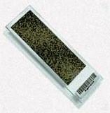
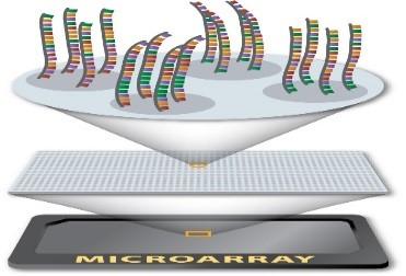
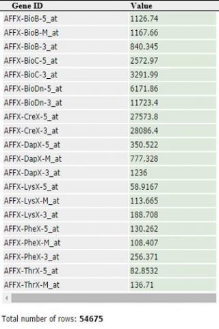
Microarray is a technology with the size of a microscope slide, or even smaller where scientists can study many genes at a time or they can learn about every gene in a single experiment. It contains thousands of spots and each spot contains the strands of DNA sequence corresponding to a single gene. The cell types can be differentiated by measuring the gene expression of different cells indicated on the microarray chip. Figures 1, 2, and 3 show the Microarray chip, structure of one spot on Microarray data and the values of each spot after scanning the Microarray chip, respectively. Generally, the dataset contains various ambiguous information in the form of missing values, outliers, inliers, etc. The microarray dataset usually contains inexpressive genes, which reduces the quality of analysis.
Figure 1. Microarray chip
Figure 2. DNA spot on microarray
Figure 3. Sample of microarray data
The complete analysis incorporates in two phases:
The complete illustration of the proposed approach is as follows.
1. Data collection: The data set for a classification model, which is used for training the models is obtained from Kent Ridge Bio-medical Data Set Repository [13].
2. Imputation of missing data and dataset normalization: The missing values of dataset are imputed using the mean value of the respective feature, then the datasets are normalized using Min-Max normalization [14].
3. Selection of relevant features: Statistical test like t-test has been applied to select the features which are expressed, and reduces the dimensions of the dataset. It results in the reduction of curse of dimensionality issue.
4. Partition of Dataset: The dataset is partitioned into two groups viz. training set and testing set using Algorithm 5.
5. Training and testing of a classifier: Different classifiers like ELM and RVM with different kernel functions are trained. The trained model is tested using the testing dataset.
6. Performance evaluation: The performance of the classifier is evaluated using precision, recall, specificity, F-Measure, ROC curve and accuracy parameters. Also “10-fold CV" is applied to validate the model, which generalizes the model. [15].
In this section, different performance metric is highlighted to measure the performance of the classifier. The confusion matrix which provides the complete statics for the correct and incorrect predictions made by a classification model compared to that of the actual samples in the dataset [16]. The confusion matrix is represented in Table 1. It is a table, which represents the prediction made by classifies which is correct and incorrect. The corresponding performance metric are shown in Table 2.
Table 1. Confusion matrix
|
Actual class |
Predicted class |
||
|
|
Negative |
Positive |
|
|
Negative |
tn |
fp |
|
|
Positive |
fn |
tp |
|
|
Performance parameters |
Description |
|
Precision $=\frac{t p}{f p+t p}$ |
It shows how much we predicted correctly out of all the classes. It should be high as possible. |
|
Recall$=\frac{t p}{f n+t p}$ |
It indicates the number of the relevant items are to be identified |
|
$F-M e a s u r e=\frac{2 * \text {Precision} * \text {Recall}}{\text {Precision}+\text {Recall}}$ |
It is defined as the harmonic mean of the precision and recall. |
|
Specificity$=\frac{t n}{f p+t n}$ |
It focuses on how effectively a classifier identifies negative labels. |
|
Accuracy$=\frac{t p+t n}{f p+f n+t p+t n}$ |
It shows on how effectively the model correctly predicts the samples. |
|
Receiver operating characteristic (ROC) curve |
ROC curve, is a graphical plot which illustrates the performance of a binary classification model when its discriminating threshold value is varied. It provides the association between “true positive rate (sensitivity)" and “false positive rate. |
In this section, various methods are selected to perform a better analysis of microarray datasets. After literature survey, it is clear that various statistical and machine learning techniques are applied as a feature selection and extraction; and for performing the classification. Here, we are applying statistic test like t-test for feature selection. Extreme Learning Machine [10] and Relevance Vector Machine [11] are applied for classification.
In this section, the obtained results are discussed for the proposed work. Three case studies viz., leukemia [13], ovarian cancer [17] and breast cancer [18] microarray datasets are applied to measure the performance of the classifier. To reduce the variances and biasness of the classifier cross validation technique is applied. Here, “10 fold cross validation (CV)" is used to generalize the model, which is able to perform better with new datasets which are completely new to the model. After identification of significantly expressed genes using t-test as a feature selection method, the classification algorithm ELM and RVM have been applied to classify the reduced dataset.
After partitioning the dataset, the model is selected by performing 10-fold cross-validation process. This is achieved by varying the parameter C and $\gamma$ in the range of [2-5, 25], where C and $\gamma$ is a regularization and kernel parameter respectively. The best model is identified by varying the value of C and $\gamma$ using Algorithm 5, N denotes the no. of fold. After validating the model in each fold using 10-fold CV the test results are collected and confusion matrix has been drawn. The analytics has been carried out on three different microarray datasets by taking into account that the number of features is varying in the multiple of five i.e., 5, 10, 15, 20, .... The proposed classifiers have been implemented using various kernel functions viz., Linear, Polynomial, RBF and Tan-sig. The values gamma ($\gamma$) and C are identified by performing the grid search in 2-5 to 25 in each fold. The values of ($\gamma$) and C in each fold are collected and taken as a median of that, which would be the final the value of $\gamma$ and C for the final model. By taking these values, we evaluate the performance of the classifier.
5.1 Results of Leukemia cancer dataset
The leukemia dataset has a dimension of 72*7129 , which contains seventy-two samples and seven thousand twenty-nine features. The dataset is categorized into two classes ALL and AML [13]. The confusion matrix has been drawn before the applying the classifiers and shown in Table 3.
Table 3. Confusion matrix for Leukemia dataset before applying classifier
|
|
ALL(0) |
AML(1) |
|
ALL(0) |
47 |
0 |
|
AML(1) |
25 |
0 |
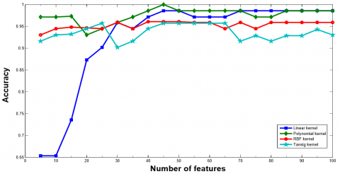
Figure 4. Classification accuracy of ELM classifier with various number of features using leukemia dataset
Table 4. Confusion matrix for ELM with different kernels on Leukemia
|
(a) Linear kernel with 45 features
|
(b) Polynomial kernel with 45 features
|
(c) RBF kernel with 40 features
|
(d) Tan-sig kernel with 45 features
|
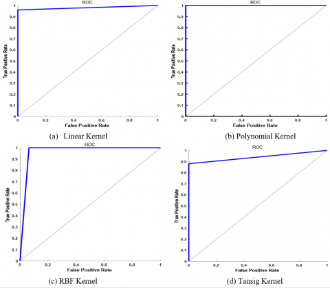
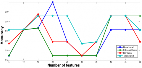
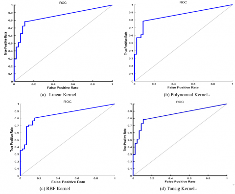
Similarly, Figure 6 shows the plot for Accuracy vs. Number of Features curve of RVM classifier with different kernels with Leukemia dataset. From Figure 6, it is imperative that maximum accuracy (minimum CV error) has been acquired when the feature set with 20, 40, 15, and 15 features are selected using RVM classifier with linear, polynomial, RBF, and tan-sig kernel function, respectively. After reaching at the highest peak the performance of the RVM classifier either degrades or remains constant. Therefore, we select the feature set with 20, 40, 15, and 15 features with linear, polynomial, RBF, and tan-sig kernel function, respectively and evaluate the rest of the performance metric. Figure 7 represents the ROC curve for RVM with different kernel using Leukemia dataset.
Table 6a, Table 6b, Table 6c, and Table 6d show the confusion matrix for leukemia data set using RVM model with various kernel functions. The rest of the performance parameters are tabulated in Table 7. The ROC curve has been plotted for RVM classifier with different kernel functions as shown in Figure 7.
Figure 6. Classification accuracy of RVM classifier with various number of features using leukemia dataset
Figure 7. ROC curve for RVM with different kernels using leukemia dataset
Table 5. Performance evaluation of ELM with various kernels Uding Leukemia
|
kernel |
Accuracy |
Precision |
Recall |
Specificity |
F-measure |
|
Linear Function |
0.9861 |
1.0000 |
0.9600 |
1.0000 |
0.9795 |
|
Polynomial Function |
1.0000 |
1.0000 |
1.0000 |
1.0000 |
1.0000 |
|
Tan-sig Function |
0.9583 |
1.0000 |
0.8800 |
1.0000 |
0.9361 |
|
Radial Basis Function |
0.9583 |
0.8928 |
1.0000 |
0.9361 |
0.9433 |
Table 6. Confusion matrix for RVM with various kernels on Leukemia dataset
|
(a) Linear kernel with 20 features
|
(b) Polynomial kernel with 40 features
|
(c) RBF kernel with 15 features
|
(d) Tan-sig kernel with 15 features
|
Table 7. Performance evaluation of kernel based RVM classifiers using Leukemia dataset
|
kernel |
Accuracy |
Precision |
Recall |
Specificity |
F-measure |
|
Linear Function |
0.9861 |
1.0000 |
0.9600 |
1.0000 |
0.9795 |
|
Polynomial Function |
0.9722 |
1.0000 |
0.9200 |
1.0000 |
0.9583 |
|
Tan-sig Function |
0.9861 |
1.0000 |
0.9600 |
1.0000 |
0.9796 |
|
Radial Basis Function |
0.9722 |
0.9600 |
0.9600 |
0.9787 |
0.9600 |
5.2 Results of Ovarian cancer dataset
The ovarian cancer dataset has a dimension of 253*15154, which contains two fifty-three samples and fifteen thousand ine hundred fifty-four features. The dataset is categorized into two classes normal and cancer [17]. The confusion matrix has been drawn before the applying the classifiers and shown in Table 8.
Table 8. Confusion matrix for Ovarian dataset before applying classifier
|
|
cancer(0) |
normal(1) |
|
cancer(0) |
162 |
0 |
|
normal(1) |
91 |
0 |
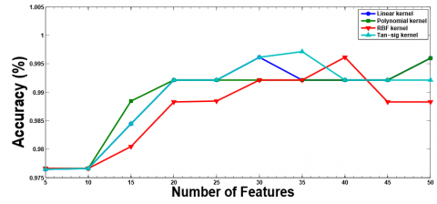
Figure 8 represents the plot for Accuracy and Number of Features curve of ELM classifier with different kernel functions. From Figure 8, it is imperative that maximum accuracy (minimum CV error) has been acquired when feature set with 50, 55, 30, and 80 features are selected using ELM classifier with linear, polynomial, RBF, and tan-sig kernel function, respectively.
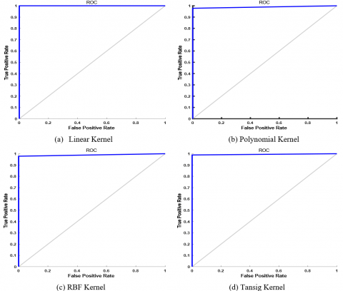
After reaching at the highest peak the performance of the ELM classifier either degrades or remains constant. Therefore, we select the feature set with 50, 55, 30, and 80 features with linear, polynomial, RBF, and tan-sig kernel function, respectively and evaluate the rest of the performance metric which is show in Table 10. The respective confusion matrix is shown in Table 9a, Table 9b, Table 9c, and Table 9d. Figure 9 represents the ROC curve for ELM with different kernel using Ovarian dataset.
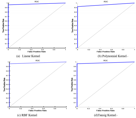
Similarly, Figure 10 represents the plot for Accuracy and Number of Features curve of RVM classifier with different kernel functions. From Figure 10, it is imperative that maximum accuracy (minimum CV error) has been acquired when feature set with 30, 50, 40, and 30 features are selected using RVM classifier with linear, polynomial, RBF, and tan-sig kernel function respectively. After attaining the peak point, the performance of the ELM classifier either degrades or remains constant. Therefore, we select the feature set with 30, 50, 40, and 30 features with linear, polynomial, RBF, and tan-sig kernel function respectively and evaluate the rest of the performance metric which is show in Table 12.
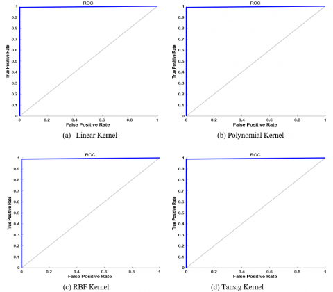
The respective confusion matrix is shown in Table 11a, Table 11b, Table 11c, Table 11d, and Table 11 show the confusion matrix for ovarian data set using RVM with various kernel methods. The plot of ROC is plotted for RVM classifier with different kernel functions as shown in Figure 11.
Figure 8. Classification accuracy of ELM with various number of features using Ovarian dataset
Figure 9. ROC curve for ELM classifier using Ovarian cancer dataset
Table 9. Confusion matrix for ELM models with different kernels using Ovarian cancer dataset
|
(a) Linear kernel with 50 features
|
(b) Polynomial kernel with 55 features
|
||||||||||||||||||
|
(c) RBF kernel with 30 features
|
(d) Tan-sig kernel with 80 features
|
Table 10. Performance analysis of kernel based ELM classifiers using Ovarian dataset
|
kernel |
Accuracy |
Precision |
Recall |
Specificity |
F-measure |
|
Linear Function |
1.0000 |
1.0000 |
1.0000 |
1.0000 |
1.0000 |
|
Polynomial Function |
0.9920 |
1.0000 |
0.9780 |
1.0000 |
0.9888 |
|
Tan-sig Function |
0.9970 |
1.0000 |
0.9890 |
1.0000 |
0.9944 |
|
Radial Basis Function |
0.9920 |
1.0000 |
0.9780 |
1.0000 |
0.9888 |
Table 11. Confusion matrix for RVM models with different kernels using Ovarian cancer dataset
|
(a) Linear kernel with 30 features
|
(b) Polynomial kernel with 50 features
|
(c) RBF kernel with 40 features
|
(d) Tan-sig kernel with 35 features
|
Figure 10. Classification accuracy of RVM with various number of features using Ovarian dataset
Figure 11. ROC curve for RVM classifier using Ovarian cancer dataset
|
kernel |
Accuracy |
Precision |
Recall |
Specificity |
F-measure |
|
Linear Function |
0.9960 |
1.0000 |
0.9890 |
1.0000 |
0.9945 |
|
Polynomial Function |
0.9960 |
1.0000 |
0.9890 |
1.0000 |
0.9945 |
|
Tan-sig Function |
0.9960 |
1.0000 |
0.9890 |
1.0000 |
0.9944 |
|
Radial Basis Function |
0.9960 |
1.0000 |
0.9890 |
1.0000 |
0.9944 |
5.3 Results of breast cancer dataset
The breast cancer dataset consists of 97 samples and 24481 features (genes). The samples are categorized as ‘relapse’ and ‘non-relapse’ classes [18]. The confusion matrix has been drawn before the applying the classifiers and shown in Table 13.
Table 13. Confusion matrix for breast cancer dataset before applying classifier
|
|
relapse(0) |
non-relapse(1) |
|
relapse(0) |
46 |
0 |
|
non-relapse(1) |
51 |
0 |
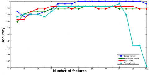
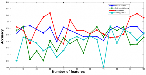
Figure 12 shows the Accuracy vs. Number of Features curve on different features for ELM Classifier with different kernel function using Breast dataset. From Figure 12, it is clear that maximum accuracy (minimum CV error) has been acquired when feature set with 15, 10, 30, and 75 features are selected using ELM classifier with linear, polynomial, RBF, and tan-sig kernel function, respectively. After attaining the peak, the accuracy of ELM classifier either degrades or remains constant. Therefore, to avoid the curse of dimensionality problem, the feature set with 15, 10, 30, and 75 features are selected using ELM classifier with linear, polynomial, RBF, and tan-sig kernel function, respectively. Table 14a, Table 14b, Table 14c, and Table 14d represent the confusion matrix for Breast dataset using ELM models. The rest of the performance parameters are tabulated in Table 15 represents the remaining parameters and Figure 13 shows the ROC curve.
Similarly, Figure 14 shows the plot of Accuracy vs. Number of Features with different features set for RVM classifier with different kernel function using Breast cancer dataset. it is clear that maximum accuracy (minimum CV error) has been attained when feature set with 5, 5, 20, and 40 features are selected using RVM classifier with linear, polynomial, RBF, and tan-sig kernel function, respectively from this figure. After attaining the highest point, the performance of RVM classifier either degrades or remains constant. Therefore, the feature set with 5, 5, 20, and 40 features are selected using RVM classifier with linear, polynomial, RBF, and tan-sig kernel function, respectively.
Table 16a, Table 16b, Table 16c, and Table 16d show the confusion matrix for Breast cancer dataset using RVM models. The rest of the parameters of performance are tabulated in Table 17. The ROC curve has been plotted for RVM classifier with different kernel functions as shown in Figure 15.
Table 14. Confusion matrix for kernel based ELM models using breast dataset
|
(a) Linear kernel with 15 features
|
(b) Polynomial kernel with 10 features
|
||||||||||||||||||
|
(c) RBF kernel with 30 features
|
(d) Tan-sig kernel with 75 features
|
Table 15. Performance analysis of kernel based ELM classifiers using Breast cancer dataset
|
kernel |
Accuracy |
Precision |
Recall |
Specificity |
F-measure |
|
Linear Function |
0.7835 |
0.7885 |
0.8039 |
0.7608 |
0.7961 |
|
Polynomial Function |
0.7835 |
0.7419 |
0.9019 |
0.6521 |
0.8141 |
|
Tan-sig Function |
0.7835 |
0.7777 |
0.8235 |
0.7391 |
0.8000 |
|
Radial Basis Function |
0.8247 |
0.8148 |
0.8627 |
0.7826 |
0.8380 |
Figure 14. Classification accuracy of RVM classifier with various number of features using Breast cancer dataset
Table 16. Confusion matrix for kernel based RVM models using Breast cancer dataset
|
(a) Linear kernel with 5 features
|
(b) Polynomial kernel with 5 features
|
(c) RBF kernel with 20 features
|
(d) Tan-sig kernel with 40 features
|
Figure 15. ROC curve for RVM classifier using breast cancer dataset
Table 17. Performance analysis of kernel based RVM classifiers using breast cancer dataset
|
kernel |
Accuracy |
Precision |
Recall |
Specificity |
F-measure |
|
Linear Function |
0.8247 |
0.8695 |
0.7843 |
0.8696 |
0.8247 |
|
Polynomial Function |
0.8454 |
0.9091 |
0.7843 |
0.9130 |
0.8421 |
|
Tan-sig Function |
0.8267 |
0.8695 |
0.8039 |
0.8478 |
0.8283 |
|
Radial Basis Function |
0.8247 |
0.8542 |
0.8039 |
0.8478 |
0.8283 |
This section presents the comparative analysis performed for the three datasets using ELM and RVM classifiers. The system configuration used in this analysis are as follows:
In this analysis, it is found that the performance (accuracy) of the four kernels varied depending on the type of data set (whether leukemia, breast or ovarian cancer) used by the two classifiers viz. ELM and RVM. So, the interpretation that can be drawn for the comparative analysis is as follows:
Table 18, Table 19, and Table 20 show the detailed comparison of ELM, RVM and SVM classifier in terms of average training, average testing accuracy and CPU time (in seconds) by considering varying numbers of feature sets. The median value of the best $\gamma$ and C from each fold is considered in both the classifiers with different kernel functions.
Table 18. Average training, average testing accuracy and CPU time (in seconds) of ELM, RVM, and SVM with different kernel functions for Leukemia dataset
|
|
Linear kernel |
Polynomial kernel |
RBF kernel |
Tansig kernel |
||||
|
ELM |
C=0.03125 |
γ = 3, C=0.03125 |
γ =2, C=0.03125 |
γ =0.0625, C=4 |
||||
|
Training Accuracy |
Testing Accuracy |
Training Accuracy |
Testing Accuracy |
Training Accuracy |
Testing Accuracy |
Training Accuracy |
Testing Accuracy |
|
|
99.69(0.0030) |
98.61(0.00063) |
100(0.0096) |
100(0.0018) |
100(0.0055) |
95.83(0.0014) |
96.44(0.0059) |
95.83(0.0013) |
|
|
RVM |
C=1 |
γ = 4 , C= 16 |
γ= 2, C= 32 |
γ = 3, C=32 |
||||
|
Training Accuracy |
Testing Accuracy |
Training Accuracy |
Testing Accuracy |
Training Accuracy |
Testing Accuracy |
Training Accuracy |
Testing Accuracy |
|
|
99.38 |
98.61(42.10003) |
98.85 |
97.22(90.52742) |
99.41 |
97.22(88.17989) |
98.85 |
98.61(39.90865) |
|
|
SVM |
C=1.5 |
γ = 3, C=32 |
γ= 8, C=32 |
γ =0.125, C=24 |
||||
|
Training Accuracy |
Testing Accuracy |
Training Accuracy |
Testing Accuracy |
Training Accuracy |
Testing Accuracy |
Training Accuracy |
Testing Accuracy |
|
|
99.69 |
100(128) |
98.3 |
98.75(218) |
99.38 |
100(114) |
100 |
100(133) |
|
Table 19. Average training, average testing accuracy and CPU time (in Seconds) of ELM, RVM, and SVM with different kernel function for breast cancer dataset
|
|
Linear kernel |
Polynomial kernel |
RBF kernel |
Tansig kernel |
||||
|
ELM |
C=0.03125 |
γ = 0.75, C=0.51563 |
γ = 0.3125, C=0.28125 |
γ = 0.046875 , C=24 |
||||
|
Training Accuracy |
Testing Accuracy |
Training Accuracy |
Testing Accuracy |
Training Accuracy |
Testing Accuracy |
Training Accuracy |
Testing Accuracy |
|
|
80.18(0.0043) |
78.35(0.00058) |
82.45(0.0058) |
78.35(0.00091) |
97.72(0.0081) |
82.47(0.0018) |
76.99(0.0083) |
78.35(0.0020) |
|
|
RVM |
C=2 |
γ = 0.0625, C= 32 |
γ = 4, C= 16 |
γ = 4, C= 16 |
||||
|
Training Accuracy |
Testing Accuracy |
Training Accuracy |
Testing Accuracy |
Training Accuracy |
Testing Accuracy |
Training Accuracy |
Testing Accuracy |
|
|
81.42 |
82.47(79.52637) |
83.29 |
84.54(64.57821) |
81 |
82.47(105.4732) |
83.29 |
82.67(95.54732) |
|
|
SVM |
C=32 |
γ = 0.125, C=32 |
γ = 1, C=4 |
γ = 0.5, C=32 |
||||
|
Training Accuracy |
Testing Accuracy |
Training Accuracy |
Testing Accuracy |
Training Accuracy |
Testing Accuracy |
Training Accuracy |
Testing Accuracy |
|
|
82.02 |
83.44(135) |
81.11 |
80.67(938) |
82.71 |
81.56(185) |
83.27 |
84.44(177) |
|
Table 20. Average training, average testing accuracy and CPU time (in Seconds) of ELM, RVM, and SVM with different kernel function for Ovarian cancer dataset
|
|
Linear kernel |
Polynomial kernel |
RBF kernel |
Tansig kernel |
||||
|
ELM |
C=0.03125 |
γ = 0.6, C=0.03125 |
γ = 0.03125, C=0.03125 |
γ = 0.03125, C=4.8 |
||||
|
Training Accuracy |
Testing Accuracy |
Training Accuracy |
Testing Accuracy |
Training Accuracy |
Testing Accuracy |
Training Accuracy |
Testing Accuracy |
|
|
100(0.019) |
100(0.0028) |
99.03(0.054) |
99.20(0.0058) |
100(0.039) |
99.21(0.0059) |
99.61(0.043) |
99.60(0.0067) |
|
|
RVM |
C=32 |
γ = 32, C=32 |
γ = 1, C=32 |
γ = 0.06255, C=32 |
||||
|
Training Accuracy |
Testing Accuracy |
Training Accuracy |
Testing Accuracy |
Training Accuracy |
Testing Accuracy |
Training Accuracy |
Testing Accuracy |
|
|
99.13 |
99.60(495.7972) |
99.61 |
99.60(305.1218) |
99.44 |
99.60(213.1664) |
99.43 |
99.60(203.2343) |
|
|
SVM |
C=32 |
γ = 32, C=32 |
γ = 1, C=32 |
γ = 0.06255, C=32 |
||||
|
Training Accuracy |
Testing Accuracy |
Training Accuracy |
Testing Accuracy |
Training Accuracy |
Testing Accuracy |
Training Accuracy |
Testing Accuracy |
|
|
99.52 |
100(146) |
99.43 |
99.23(171) |
99.86 |
100(720) |
99.77 |
84.44(177) |
|
In this paper, a classification framework was designed using ELM and RVM classifier with various kernels to classify the microarray datasets. t-test was applied to select the significant features. To enhance and generalize the model behavior 10-fold CV technique was applied. Various performance metric is applied to evaluate the classifier performance on the microarray datasets. From the computed results, it is observed that ELM with RBF kernel and RVM with polynomial kernel as classifier yields better result. Further, we can apply various meta-heuristic techniques with the relevant classifiers to make the ensemble techniques to make a better classifier. This hybridization may help in reducing the complexity of the classification model.
[1] Gao, L.Y., Ye, M.Q., Lu, X.J., Huang, D.B. (2017). Hybrid method based on information gain and support vector machine for gene selection in cancer classification. Genomics, Proteomics & Bioinformatics, 15(6): 389-395. https://doi.org/10.1016/j.gpb.2017.08.002
[2] Heller, M.J. (2002). DNA microarray technology: Devices, systems, and applications. Annual Review of Biomedical Engineering, 4(1): 129-153. https://doi.org/10.1146/annurev.bioeng.4.020702.153438
[3] He, J.X., Gao, Y., Wu, G., Lei, X.M., Zhang, Y., Pan, W.K., Yu, H. (2018). Bioinformatics analysis of microarray data to reveal the pathogenesis of brain ischemia. Molecular Medicine Reports, 18(1): 333-341. https://doi.org/10.3892/mmr.2018.9000
[4] Chow, Y.T., Darbon, J., Osher, S. and Yin, W.T. (2019). Algorithm for overcoming the curse of dimensionality for state-dependent Hamilton-Jacobi equations. Journal of Computational Physics. https://doi.org/10.1016/j.jcp.2019.01.051
[5] Rueda, L. (2019). Microarray Image and data Analysis: Theory and Practice. CRC Press.
[6] Sharbaf, F.V., Mosafer, S., Moattar, M.H. (2016). A hybrid gene selection approach for microarray data classification using cellular learning automata and ant colony optimization. Genomics, 107(6): 231-238. https://doi.org/10.1016/j.ygeno.2016.05.001
[7] Motieghader, H., Najafi, A., Sadeghi, B., Masoudi-Nejad, A. (2017). A hybrid gene selection algorithm for microarray cancer classification using genetic algorithm and learning automata. Informatics in Medicine Unlocked, 9: 246-254. https://doi.org/10.1016/j.imu.2017.10.004
[8] Zhang, Y., Li, A., Peng, C., Wang, M.H. (2016). Improve glioblastoma multiforme prognosis prediction by using feature selection and multiple kernel learning. IEEE/ACM Transactions on Computational Biology and Bioinformatics, 13(5): 825-835. https://doi.org/10.1109/TCBB.2016.2551745
[9] Sheskin, D.J. (2003). Handbook of Parametric and Nonparametric Statistical Procedures. CRC Press.
[10] Huang, G.B., Wang, D.H., Lan, Y. (2011). Extreme learning machines: A survey. International Journal of Machine Learning and Cybernetics, 2(2): 107122. https://doi.org/10.1007/s13042-011-0019-y
[11] Tipping, M. (2003). Relevance vector machine. US Patent 6,633,857.
[12] Schölkopf, B., Smola, A., Müller K.R. (1998). Nonlinear component analysis as a kernel eigenvalue problem. Neural Computation, 10(5): 1299-1319. https://doi.org/10.1162/089976698300017467
[13] Golub, T.R., Slonim, D.K., Tamayo, P., Huard, C., Gaasenbeek, M., Mesirov, J.P., Coller, H., Loh, M., Downing, J.R., Caligiuri, M.A., Bloomfield, C.D., Lander, E.S. (1999). Molecular classification of cancer: Class discovery and class prediction by gene expression monitoring. Science, 286(5439): 531-537. https://doi.org/10.1126/science.286.5439.531
[14] Jain, Y.K., Bhandare, S.K. (2011). Min max normalization based data perturbation method for privacy protection. International Journal of Computer & Communication Technology (IJCCT), 2(8): 45-50.
[15] Kumar, M., Rath, S.K. (2014). Classification of microarray data using kernel fuzzy inference system. International Scholarly Research Notices, 2014(Article ID 769159): 18 pages. https://doi.org/10.1155/2014/769159
[16] Catal, C. (2012). Performance evaluation metrics for software fault prediction studies. Acta Polytechnica Hungarica, 9(4): 193-206.
[17] Petricoin, E.F. III, Ardekani, A.M., Hitt, B.A., Levine, P.J., Fusaro, V.A., Steinberg, S.M., Mills, G.B., Fishman, C.D.A., Kohn, E.C., Liotta, L.A. (2002). Use of proteomic patterns in serum to identify ovarian cancer. The Lancet, 359(9306): 572-577. https://doi.org/10.1016/S0140-6736(02)07746-2
[18] Veer, L.J., Dai, H., Vijver, M.J., He, Y.D., Hart, A.M., Mao, M., Peterse, H.L., Kooy, K.V., Marton, M.J., Witteveen, A.T., Schreiber, G.J., Kerkhoven, R.M., Roberts, C., Linsley, P.S., Bernards, R., Friend, S.H. (2002). Gene expression profiling predicts clinical outcome of breast cancer. Nature, 415(6871): 530-536. https://doi.org/10.1038/415530a
[19] Sachan, V., Kumar, I., Sankar, R., Mishra, R.K. (2018). Analysis of transmit antenna selection based selective decode forward cooperative communication protocol. Traitement du Signal, 35(1): 47-60. https://doi.org/10.3166/TS.35.47-60
[20] Kumar, K., Mishra, R.K. (2019). A robust mRMR based pedestrian detection approach using shape descriptor. Traitement du Signal 36(1): 79-85. https://doi.org/10.18280/ts.360110