Sarah Adnan Saeed | Israa Kh. Jasim | Anwer M. Ali*
© 2026 The authors. This article is published by IIETA and is licensed under the CC BY 4.0 license (http://creativecommons.org/licenses/by/4.0/).
OPEN ACCESS
The purpose of this study is to develop a precise predictive model to estimate the Indirect Tensile Stiffness Modulus (ITSM) of fiber-reinforced cold mix asphalt (FRCMA) using Artificial Neural Networks (ANNs). Two ANN architectures, ANN-I with a compact (3 nodes) configuration in the hidden layer and ANN-II with an expanded configuration (6 nodes) in the hidden layer, were trained on an extensive database consisting of experimental mix designs with varying fiber types, contents and treatment, curing time (CT), and environmental conditions. The models were developed using SPSS Modeler and evaluated with several statistical metrics such as Root Mean Square Error (RMSE), Coefficient of Determination (R²) and Mean Absolute Percentage Error (MAPE). The ANN-II produced better predictive performance than the ANN-I, having a MAPE of 59.46% and R² of 0.956, compared to the ANN-I’s MAPE of 66.61% and R² of 0.913. Sensitivity analysis identified CT, humidity condition (HC) and air void content (%AV) as the three strongest predictors of ITSM. The relatively high MAPE does indicate that prediction error remains substantial; however, the ANN predicts the general nonlinear trends of eco-friendly fiber-reinforced asphalt concrete (ECC) fairly adequately with its single-output architecture. As such, the model created may prove to be a useful tool for pavement engineers, while further developing and obtaining larger-sized data will improve model accuracy.
Artificial Neural Networks, fiber-reinforced cold mix asphalt, Indirect Tensile Stiffness Modulus, fiber reinforcement, predictive modeling
A significant number of studies have focused on the search for sustainable and cheaper alternatives to the hot mix asphalt (HMA). Most of them look into the cold mix asphalt (CMA) technology. Cold asphalt mixes are produced and applied at room temperature, so that they reduce the energy consumption and greenhouse gas emissions dramatically. It is worth noting that these mixes reduce fuel consumption and, thus, the production and operational costs [1, 2]. Therefore, when heating equipment is not available or practical, these mixtures are highly profitable for the construction operations of maintenance activities held in remote construction areas. However, CMA has witnessed historical mechanical underperformance compared to HMA; hence, attributes like stiffness, cohesion, and moisture susceptibility are some of which are found wanting [3], and thus deny it widespread use in the structural layers of the pavements.
To surpass these limitations, the proficiency of CMA has been reinforced with fibers through the research documented in the references [4, 5]. The tensile properties, crack resistance, and long-term durability tend to improve due to fibers such as synthetic fibers, polyester, and polypropylene, which can enhance the stress distribution and removal of premature distress; coir fibers and jute fibers can produce a less effective enhancement, as natural fibers give the environmentally helpful ability [6]. Additional fibers will also improve the stiffness and toughness of cold mixes, reduce crack propagation, and increase post-peak load-bearing strength [7].
While it is evident that fiber reinforcement offered a great amount of promise, accurately predicting the Indirect Tensile Stiffness Modulus (ITSM) of fiber-reinforced cold mix asphalt (FRCMA) still remains a challenge for a number of reasons. Such reasons include but are not limited to the material’s nonlinear behavior, complex nature, and sensitivity to curing conditions and mix design variables – all of which make relationships hard to describe mathematically. Although for quite a long time, regression-based models have been developed in order to try and pin down relationships of this kind, these have proven to falter where intricate relationships of this kind are concerned. This is why artificial intelligence techniques have come into the frame to a greater extent, to date. Of these, Artificial Neural Networks (ANNs) are among the most-used when it comes to modeling the behavior of composite materials [8, 9].
ANNs are capable of modeling and implementing the way the brain learns to find or classify patterns, models, and rules in large and complicated datasets. By using ANNs to represent non-linear relationships, there is significant potential to develop ANN models without the need for a priori equations, as is the case with pavement performance parameters, which have a variety of complex and multi-dimensional interrelated factors affecting their performance [10]. Research supporting the use of ANNs to predict asphalt mixture stiffness [11], as well as to determine the compressive strength of concrete [12], and to predict the operation of reservoir facilities [13], ANN configurations like multilayer perceptron (MLP) architectures that have been trained to identify patterns using backpropagation (BP) algorithms can demonstrate a greater level of flexibility and plasticity in their ability to predict the behaviour of materials with respect to the various inputs that can be used to predict material behaviour [14, 15].
The primary goal of the current research is to create ANN models to forecast the ITSM of FRCMA mixtures using experimental data. Two different multi-input single-output ANN architectures were constructed and tested, denoted as ANN-I and ANN-II, which had identical input/output structures, but differed exclusively in the number of neurons in the hidden layer. The purpose of this design was to evaluate the influence of hidden layer size on the predictive accuracy of ITSM. This study makes four main contributions, as follows: (i) development of ANN-based predictive models for measuring the ITSM of fiber-reinforced CMA mixtures; (ii) inclusion of mixture-related, curing-related and environmental variables, such as fiber type, blend ratio, content, length, humidity, curing time (CT) and void content, in the ANNs; (iii) preparation of the appropriate encoding for categorical variables to avoid a false numerical ordering in ANN training; and (iv) comparison of predictive performance for the two ANN architectures using appropriate statistical performance measures to determine the suitability for engineering predictive modelling of ITSM.
The remaining sections of this study are as follows: Section 2 consists of details surrounding the dataset, the input/output variables, the categorical variable encoding approach, ANN model creation, and an example methodology to evaluate ANN performance. Section 3 describes the database used in this study. Section 4 details the study methodology and experimental setup. Section 5 provides prediction data and statistical performance results for both ANN-I and ANN-II. Section 6 concludes the study with a summary of key findings and recommendations for future research.
Functioning like a biological neuron connecting with other neurons by transmitting numerical information through weighted connections [16], ANNs work as interconnected units. For modelling material behaviour, such as ITSM prediction of CMA, ANNs have a strong ability to generalize from input-output datasets. Fiber type 1 (FT1), fiber type 2 (FT2) and the blend ratio (FT1/FT2) are fiber types, and fiber content by aggregate weight (%FC) can be considered as the inputs in this study. Also, fiber length (FL), air void content (%AV), CT, and humidity condition (HC) can act as the input variables in this study. However, ITSM is used as the output variable.
Choosing an appropriate network architecture and adequately training and validating the ANN model are particularly important aspects to create a reliable ANN model [15]. An architecture includes an input layer, 1 or more hidden layers, and an output layer. The architecture decides its performance and usually depends upon the number of layers, the number of neurons in different layers, and the activation function [17]. In this study, A back-propagation network back-propagates the error to train the ANN model to update the weights using the gradient descent method. The accuracy of the model widely depends on the hyperparameters of the ANN model. Depend on the learning rate, hidden neurons, and the number of training data in the ANN model [18]. Through tuning and validation, it was optimized.
SPSS Modeler was chosen due to its user-friendly interface and robust analytics that proved to afford an adaptable network structure and easy model performance evaluation across different configurations.
The predictive capacity of ANNs depends on the quality and diversity of the training dataset. A representative and structured dataset helps the model to understand complex and non-linear relationships between the inputs and outputs, resulting in better predictive performance [15, 16]. For this research, one dataset has been compiled to train and validate the ANN models for the estimation of ITSM of fiber-reinforced cold-mix asphalt. The first dataset is comprised of 68 unique CMA mixtures that were collected from the published peer-reviewed papers focusing on fiber reinforcement and mechanical performance under different curing and moisture conditions [2, 19-23], and totaling 123 mix designs, as presented in Table 1, where some variables are qualitative variables like fiber type and HC.
Table 1. Definition of variables used in the Artificial Neural Networks (ANNs) model for cold mix asphalt (CMA)
|
Symbol |
Variable Type |
Description |
Range |
Unit |
Treatment in ANN Model |
|
ITSM |
Output |
Indirect Tensile Stiffness Modulus (MPa) |
17.12–2208 |
MPa |
Single target output variable |
|
FT1 |
Categorical input |
Fiber Type 1 (0 = No fiber, 1 = Cellulose, 2 = Glass, 3 = Nylon, 4 = Polyester, 5 = Basalt, 6 = Hemp, 7 = Jute, 8 = Coir) |
0–8 |
Range |
Treated as a nominal categorical variable and transformed using one-hot/dummy encoding |
|
FT2 |
Categorical input |
Fiber Type 2 (0 = No fiber, 1 = Cellulose, 2 = Glass, 3 = Nylon, 4 = Polyester, 5 = Basalt, 6 = Hemp, 7 = Jute, 8 = Coir) |
0–8 |
Range |
Treated as a nominal categorical variable and transformed using one-hot/dummy encoding |
|
FT1/FT2 |
Continuous input |
Fiber Blend Ratio by Mass (FT1:FT2) |
0–1 |
% |
Continuous numerical input |
|
%FC |
Continuous input |
Fiber Content (% by weight of total aggregate) |
0–0.55 |
% |
Continuous numerical input |
|
FL |
Continuous input |
Fiber Length |
0–20 |
mm |
Continuous numerical input |
|
HC |
Binary categorical input |
Humidity Condition (1 = Dry, 2 = Wet) |
1–2 |
Range |
Recoded as a binary input variable |
|
CT |
Continuous input |
Curing Time (days) |
1–360 |
days |
Continuous numerical input |
|
%AV |
Continuous input |
Air Void Content |
18.8–26.3 |
% |
Continuous numerical input |
The following variables were used to develop ANN models for predicting ITSM of FRCMA mixtures (see Table 1). The dataset contains continuous numerical variables and categorical variables. In preparation for ANN training, the categorical variables were encoded to prevent treating the numerical labels of the categorical variables as continuous or ordinal values.
The fiber-type variables FT1 and FT2 are categorical (i.e., nominal) variables and were originally identified using a numerical system that had been assigned from 0 to 8. These numbers were only to serve as identifiers of the specific categories that they represented, and should not have been entered into the ANN models as numerical input. Rather, they were converted using a one-hot/dummy coding procedure so that each fiber type was represented with a separate binary indicator variable. This method will also prevent the ANN from assigning any type of false rank or distance to the different fiber types.
HC was recoded as a binary variable, where dry and wet conditions were represented using binary coding. The other input variables in the original dataset constituted as continuous (continuous data), while the remaining variables were converted into dummy variables via first order effects from FT1 and FT2 via one-hot encoding; thus the last (input) vector to create the final (input) dataset was an association of all continuous variables, one-hot/dummy FT1/FT2 variables, as well as binary coded HC variable. The table contains records of encoded input used (in accordance with ANN-I/II in the evaluation protocol & provided in Section 1, ANN Development) to build models based on the included ANN-I/II, respectively.
IBM SPSS Modeler version 23, 2024, was used to perform categorical encoding. The Type node identified FT1 and FT2 as nominal input variables and HC as a binary/flag input variable. The Derive node generated dummy variables for FT1 and FT2. The Filter node removed the original FT1 and FT2 input variables from being included as input in the ANN model. The ANN models were trained by using the correctly encoded input.
Due to the inclusion of categorical fiber type variables, hybrid fiber combinations, and disparate experimental areas in the present dataset, in which many possible combinations will never be able to occur, a traditional multiple linear regression model was not used as a baseline in this study. Therefore, it is not expected that a simple linear continuous relationship will exist between the independent variables and ITSM. ANN was chosen to model the nonlinear relationships and complex interactions of the independent variables in this study (fiber type, fiber blend ratio, fiber content, FL, HC, CT, and %AV). Because of this, the current study focused on the evaluation of ANN-based predictions of ITSM. Future researchers are strongly encouraged to utilize a wider variety of comparison baseline models and other machine learning techniques.
All ITSM records in the compiled database were screened and cleaned prior to the development of models in order to ensure integrity. In developing models, we excluded records with missing output values or with incomplete essential input data. For records that had one or two missing input values only, statistical imputation was employed to fill in the missing data points. Group-wise mean or median imputation was used if the surrounding records had similar fiber type, fiber content, CT, %AV, and mixture characteristics; where appropriate, nearest neighbor imputation was also employed. The testing conditions as indicated for each of the testing locations included: temperature; loading procedure; geometry of the test specimen; and testing standards; to the extent that this information was made available, increased cross-paper comparability of test results was accomplished. However, because of inconsistency in reporting test protocol details across source studies, there will still be possible inter-study variability. Therefore, the source paper was left in as a grouping factor for leave-one-study-out validation to see if the accuracy of the model is governed by material behavior rather than being specific to the conditions of the testing.
The selection and consistency of input parameters play a critical role in developing a reliable ANN model for predicting mechanical performance. In the current study, all neural network models were developed using fixed input variables across all phases of training and testing. These included FT1, FT2, FT1/FT2, %FC, FL, CT, HC, and %AV, while the output variable was the ITSM.
The ITSM of FRCMA was estimated using two different ANNs with the same structure, consisting of multiple inputs and a single output. The input variables and the output variable are referred to in Table 1. The two networks consisted of the same number of inputs and output variables; however, the function associated with the output variable was unique for each network, and the only difference between ANN-I and ANN-II was that ANN-I had 3 neurons in the hidden layers while ANN-II was fitted with 6 neurons in the hidden layers. The number of neurons in the hidden layers was established through an iterative trial-and-error method by testing a number of neurons from a range of 1 to 17, in order to find an acceptable range of architectures that provided the lowest training error and highest correlation coefficient between ANN outputs and predicted ITSMs. Thus, ANN-I and ANN-II were used for comparison to determine the effect of hidden layer neuron count on the prediction accuracy of ITSMs without assigning hidden layer neurons separately to each individual architecture of the fiber. The evaluation of the ANN models was provided through a fixed training-validation-testing protocol to prevent any optimistic performance estimates and any data leakage. The ANN models used the training set for model fit; the validation set was used only for selecting model architecture and controlling those selection processes during the trial-and-error phase. The test set was independent from all data used for the selection of: 1) the data split; 2) the ANN architecture; 3) the tuning of hyperparameters; 4) the preprocessing decisions; and 5) any decisions related to stopping rules, followed by developing ANN-I or ANN-II architectures. The final test set was used only once to report the final predictive performance for ANN-I and ANN-II architectures after they were locked.
The testing sample that was used for performing all tests, such as data splitting for determining test set size, selecting architecture, hyperparameter tuning, making choices regarding pre-processing of data, and stopping rule decisions, was not used as the basis for selecting any of these parameters prior to its use for reporting the final predictive performance on both the ANN-I and ANN-II architectures after their locking step.
The locked neural network (ANN) architectures, as well as how they would be evaluated (testing), for ANN-I and ANN-II, are summarized in Table 2. The only difference between the two networks was the number of neurons in the hidden layer; ANN-I had 3 hidden neurons, while ANN-II had 6 hidden neurons. The published testing results were based on holding out an independent test set from the validation set and only after the model selection procedure was completed on the validation set. The best number of nodes in the hidden layer in the ANN-I model was three nodes and for the ANN-II model, it was six nodes in its hidden layer.
Table 2. Data division ratios on ANN-I and ANN-II model performance for fiber-reinforced cold mix asphalt (FRCMA)
|
Model |
ANN-I |
ANN-II |
|
Input Layer |
8 |
8 |
|
Hidden Layer |
3 |
6 |
|
Output Layer |
1 |
1 |
|
Training (%) |
90 |
89 |
|
Validation (%) |
2 |
3 |
|
Testing (%) |
8 |
8 |
|
Training Error (%) |
5.2 |
2.5 |
|
Final Test Error (%) |
3.26 |
2.3 |
|
Correlation, r (%) |
95.1 |
97.8 |
|
Training Set Use |
Model fitting |
Model fitting |
|
Validation Set Use |
Architecture selection and stopping control |
Architecture selection and stopping control |
|
Test Set Use |
Final performance reporting only |
Final performance reporting only |
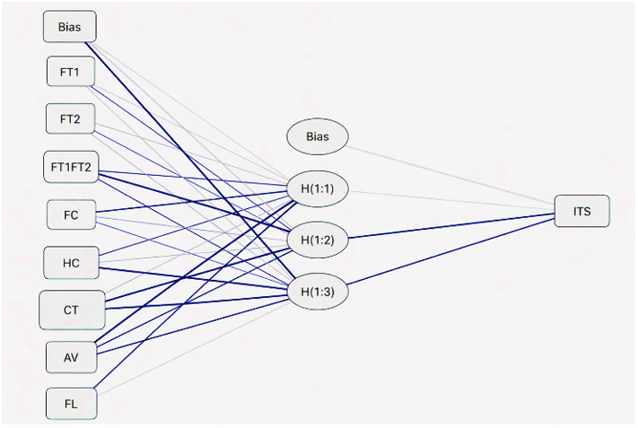
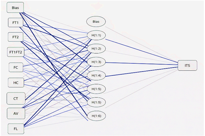
The reported training and final test errors represent the relative prediction error (%) calculated between the observed and predicted ITSM values; they are not RMSE or MAPE values. The first approach, referred to as ANN-I, utilized a multi-input, single-output structure configuration and three nodes in the hidden layer to predict the ITSM responses across various fiber combinations simultaneously from a single network. This architecture was trained exclusively using a dataset collected from previous studies, which consists of a broad range of CMA formulations with varying fiber modifications. The second approach, labeled ANN-II, followed a multi-input, single-output structure and six nodes in the hidden layer. This allowed for a more focused prediction of ITSM for each mix variation.
Figure 1. Architecture of neural network model for ANN-I
Training both ANN models was accomplished by using the Levenberg–Marquardt BP algorithm, which was implemented through its default system parameters available in SPSS Modeler, which was used to develop and train the neural network in this study. This algorithm was chosen due to its simplicity and effectiveness in nonlinear regression problems, as it has been successfully used for providing optimal design input in pavement engineering circumstances where relationships (input-output) are complicated [15]. The architecture of ANN-I and ANN-II is shown in Figures 1 and 2, respectively. The hyperbolic tangent (tanh) function was applied as an activation function in the hidden layer of the network. The training procedure was implemented according to the algorithm and optimization settings available within the selected SPSS Modeler neural network configuration. The applied settings included the network architecture, hidden-layer structure, activation functions, error function, maximum number of training cycles, and stopping criteria. These settings were used to control the model training process and reduce prediction error during the learning phase. Also, the Levenberg–Marquardt optimization algorithm was used for network training; therefore, learning-rate and momentum parameters were not applied.
Figure 2. Architecture of neural network model for ANN-II
In order to appraise the precision and adequacy of the refined ANN models for forecasting ITSM of FRCMA, Comparative analysis between the predicted and the actual experimental values were reached based on a number of well-known statistical indices and performance criteria, which are namely, Root Mean Square Error (RMSE), Normalized Root Mean Square Error (NRMSE), Mean Absolute Percentage Error (MAPE), Coefficient of Determination (R²), and Pearson Correlation Coefficient (R).
The expressed statistical term, RMSE, in Eq. (1) explains how far off the ITSM values are off by contrasting it to the actual (An) and predicted (Pn) values and comparing the estimated (predicted – or Pn) ITSM (P) values across the N number of points within the dataset with the true (actual – or An) ITSM (A) values for the dataset. Consequently, the lower the RMSE, the more reliable the equation.
$R M S E=\sqrt{\frac{1}{N} \sum_{n=1}^N\left(A_n-P_n\right)^2}$ (1)
In order to make it comparable across models and datasets, the RMSE was normalized against the mean of the actual values ($\overline{{A}}$) to give NRMSE, as shown in Eq. (2). Such normalization becomes essential, as otherwise RMSE will be incomparable when the datasets have different scales or different units.
$N R M S E=\frac{R M S E}{\overline{\mathrm{~A}}}$ (2)
where, $\overline{{A}}$ is the mean of the average ITSM values. Additionally, the proportion of variation in ITSM that is captured by the model predictions was assessed by the R², which is given in Eq. (3). An R² nearing 1 indicates a good model accuracy, whereas values around 0 suggest poor prediction [15].
$R^2=1-\frac{\sum\left(A_n-P_n\right)^2}{\sum\left(A_n-S_n\right)^2}$ (3)
where, An is the actual ITSM value, Pn is the predicted ITSM value, and Sn is the mean of the actual ITSM values. Similarly, the predictive accuracy of the methods was gauged using the MAPE, which automatically expresses the prediction error as a percentage.
MAPE $=\frac{100}{N}\left(\sum \frac{\left|A_n-P_n\right|}{A_n}\right)$ (4)
The R is a measure of the linear relationship between the predicted values of ITSM and the actual values observed. R values greater than (closer to 1) indicate a strong positive correlation between the predicted and observed ITSM values.
To investigate the impact of the material consistency on the model’s prediction performance, the ANN-I and ANN-II architectures were applied for a homogenous dataset, which was collected [20], consisting of ten CMA samples that include fiber additives from a controlled source. The dataset was selected due to reduced data consistency since it was considered an ideal definition for assessing the sensitivity of the model's performance to the input consistency. Therefore, for testing the model consistency and prediction accuracy, the RMSE, NRMSE, MAPE, R², and R values are calculated and discussed.
Two network structures have been designed and constructed, which are capable of modeling the ITSM of FRCMA by ANN. Multiple research data sets were used to train and optimize those two network structures.
5.1 ANN-I model
To create and grasp the full independence of the ANN-I, a model was generated and trained using different sorts and states of the FRCMA mixtures. Particularly, the technique was evaluated by using ANNs on data from up to 31 material sources and 8 material fiber types (both straight and hybrid). Evaluation of the procedure is performed through a mixture of visual diagnostics for making analysis, as well as introducing some statistical indicators, including R², RMSE, NRMSE, MAPE, and the correlation value R.
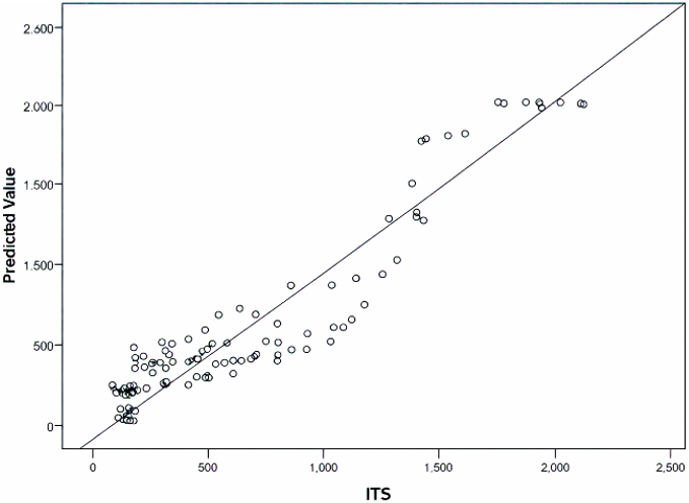
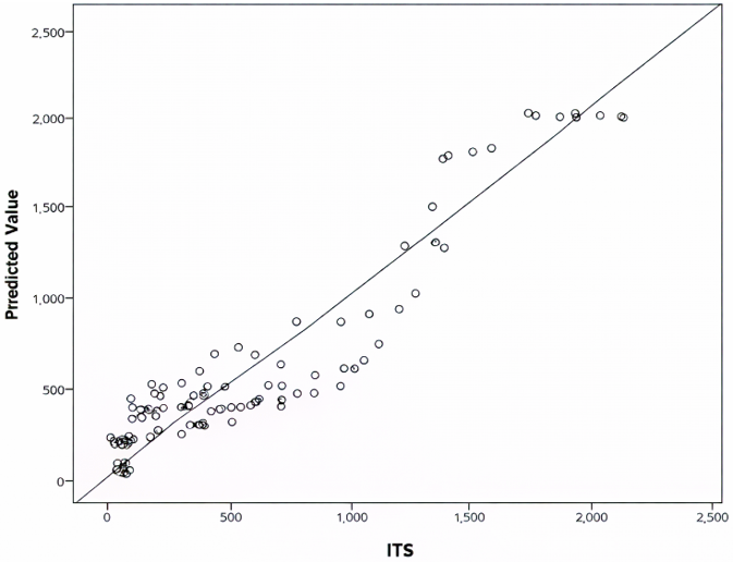
An evident depiction, as shown in Figure 3, is the scatter plot of the predicted and the actual values of the ITSM; they all follow a flexible pattern, each with a few outliers and again aligned with the 1:1 reference line, which portrays that the predictions match the actual values in the mid to high stiffness regions. However, deviation becomes more noticeable at lower ITSM values, suggesting reduced model accuracy for softer mixes.
Figure 3. Scatter plot of actual vs. predicted Indirect Tensile Stiffness Modulus (ITSM) values using ANN-I
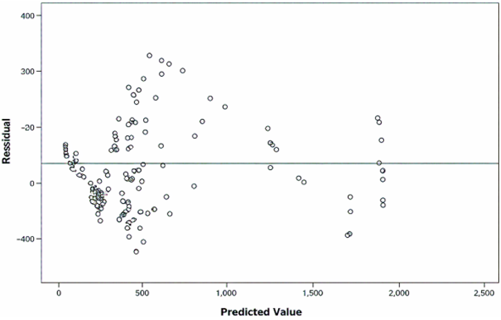
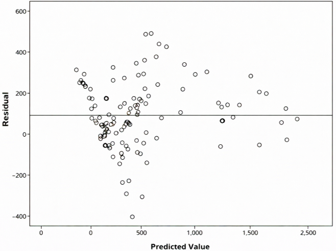
Figure 4. Residual distribution plot for ANN-I predicted Indirect Tensile Stiffness Modulus (ITSM)
The distribution of residuals shown in Figure 4 indicates that mixtures with very short CT, or mixtures without fiber reinforcement, were biased toward an underprediction of results within the lower stiffness range (i.e., less than 400 MPa) of the residuals.
The ANN-I architecture computed an RMSE value of 174.85 MPa, as shown in Table 3, which corresponded to a Normalized RMSE (NRMSE) level of 32.2%, thus indicating a moderate degree of predicted values that are dispersed relative to the overall mean actual ITSM value. The MAPE value was 84.83%, representing a relatively high average deviation in percentage terms. However, this value should be interpreted with caution because MAPE is highly sensitive to small actual ITSM values and may overestimate the relative error when the denominator is low.
Table 3. Performance evaluation indicators of the ANN-I model
|
Performance Indicator |
Value |
|
Root Mean Square Error (RMSE) |
174.85 MPa |
|
Normalized RMSE (NRMSE) |
32.2% |
|
Mean Absolute Percentage Error (MAPE) |
84.83% |
|
Coefficient of Determination (R²) |
0.903 |
|
Pearson Correlation Coefficient (R) |
0.951 |
To provide a more robust assessment of prediction error, additional indicators, including Mean Absolute Error (MAE) and a robust percentage-based metric such as Symmetric Mean Absolute Percentage Error (SMAPE) or Median Absolute Percentage Error (MdAPE), should be reported. Moreover, the prediction errors should be further examined within different ITSM ranges, such as <400 MPa, 400–800 MPa, and >800 MPa, to clarify whether the high percentage error is mainly associated with low-stiffness mixtures.
Yet, the ANN-I model also exhibits a strong relationship between predicted and actual values, with an R² value of 0.903 and Pearson's coefficient of correlation equal to 0.951. This indicates that the ANN-I model successfully captured the overall trend of the ITSM data, although its magnitude-based prediction accuracy requires further improvement, particularly for mixtures with low ITSM values.
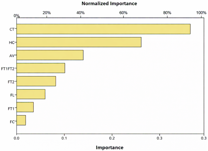
Figure 5. Normalized importance of input variables in Indirect Tensile Stiffness Modulus (ITSM) prediction
Figure 5 shows the results of the feature importance analysis for input features affecting ITSM results. CT contributes the most significant impact, HC is the second strongest contributor, and %AV the third. This helps to confirm that environmental and time-dependent curing impacts are significant when assessing the ability of a mix or binder to provide a stiff asphalt. There were also moderate levels of contribution from FT1/FT2 and FT2, while FT1, FL, and %FC have only a minimal impact, most likely due to the narrow range of values for these parameters in the dataset.
The ANN-I model does provide an accurate prediction correlation of ITSM based primarily on the relatively homogeneous curing characteristics used in the training dataset; however, the model will be improved by using a more diverse training dataset and focusing on optimizing prediction performance within the lower stiffness ranges. Future research should include a larger distribution of input parameters and should also investigate the effect of parameter interactions to improve prediction accuracy.
5.2 ANN-II model
The ANN-II model was developed and trained using the same data structure as ANN-I. However, both ANN-I and ANN-II used a multi-input, single-output structure. Therefore, the main difference between the two models was the number of neurons in the hidden layer, where ANN-I had 3 hidden neurons while ANN-II had 6 hidden neurons. The evaluation of the ANN-II model was performed with graphical and statistical techniques in order to determine its accuracy and ability to generalize.
Figure 6. Scatter plot of actual vs. predicted Indirect Tensile Stiffness Modulus (ITSM) values using ANN-II
Figure 7. Residual distribution plot for ANN-II predicted Indirect Tensile Stiffness Modulus (ITSM)
The scatter plot of ITSM actual values and predicted values, as shown in Figure 6, indicates a significant degree of alignment in the actual vs. predicted values, especially over the full range of stiffnesses. The data points fall very close to the 1:1 reference line for most of the range, with far fewer deviations from the reference line at the lower stiffness values than ANNI. The results indicate that the single-output ANN-II model provides better calibrated results throughout the entire range of responses.
The improved predictive performance is confirmed by the residual distribution shown in Figure 7. While there are still some residuals dispersed across these ranges of stiffness, they are now distributed more equally about zero and are indicative of less systematic bias than before.
The ANN-II model was able to quantitatively outperform the ANN-I model, but this can only be done with more precision than what can be verified using statistical validity. The RMSE of 118.00 MPa and NRMSE of 21.74% demonstrate that there was a moderate amount of error in terms of prediction on the ITSM scale, so while the model is suitable for use as a basis to compare mixtures of different types, it would not be appropriate to use it as the sole source of information on how much material to use in a specific mix design. The MAPE of 59.46% demonstrates that the accuracy of individual predictions by the model may still be large; however, those measures were improved compared to the ANN-I model. The model R² value of 0.956 and R of 0.978 indicate that the ANN-II model is in excellent agreement with the measured/modeled values. As such, in order to validate the benefits attributed to the ANN model, a comparison should be made to a linear multiple regression model.
A multiple linear regression was run as the baseline to determine if it was necessary to use an ANN or not. The ANN-II model will only be determined to be better than the baseline regression if it has lower RMSE and NRMSE than the baseline regression and higher R² and Pearson R than the baseline regression. The comparison of these results will show that the ANN model is able to capture the nonlinear effects that cannot be properly modeled with a simple linear regression.
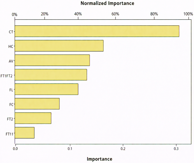
Figure 8. Normalized importance of input variables in ANN-II
As demonstrated through Figure 8, CT was once again determined to be the most significant predictor, followed by HC and the %AV (Similar to the ranking established by ANN-I). However, when reviewing the variable importance in ANN-II, it seems that the importance of fiber-related variables, such as %FC and FT1/FT2, may be a bit stronger due to the blown learning structure with reduced noise resulting from multiple outputs of a given variable.
By demonstrating improved predictive performance, less residual variance, and a more balanced distribution of sensitivity across the input feature space, ANN-II offers several advantages over its predecessor, ANN-I. The findings of this study imply an appropriate means by which to model ITSM accurately through a single-output ANN framework, particularly when data are heterogeneous and/or localized prediction control is necessary.
5.3 Effect of hidden layer nodes for ANN-I and ANN-II
A significant difference in the underlying architectures of ANN-I and ANN-II is the manner in which the output structure is associated with the hidden layer nodes in ANN-I. Predominantly, ANN-I has been developed to allow for one-to-one mapping (single-output model) from a single network for all ITSM predictions made. However, this design allows for a leaner architecture, often requiring fewer neurons in the hidden layer, as the network focuses solely on one output-target relationship per training session.
In contrast, ANN-II follows a single-output configuration, where each ITSM value is predicted independently using a dedicated network. As a result, ANN-II benefits from reduced training noise, more stable weight updates, and improved convergence, leading to significantly better performance reflected in Table 4.
Table 4. Performance evaluation indicators of the ANN-II model
|
Performance Indicator |
Value |
|
Root Mean Square Error (RMSE) |
118.00 MPa |
|
Normalized RMSE (NRMSE) |
21.74% |
|
Mean Absolute Percentage Error (MAPE) |
59.46% |
|
Coefficient of Determination (R²) |
0.956 |
|
Pearson Correlation Coefficient (R) |
0.978 |
Empirically, ANN-II not only demonstrated lower RMSE and MAPE values but also outperformed ANN-I in correlation-based metrics (R² and Pearson R), indicating that simplifying the model to single-output pathways helped the network better capture the underlying patterns in the ITSM prediction task.
The number of nodes in the hidden layer should be context-sensitive: single-output models like ANN-I and ANN-II, where single-output designs can often achieve higher accuracy with fewer, more focused neurons when the dataset supports such separation.
[1] Zaumanis, M., Mallick, R.B. (2015). Review of very high-content reclaimed asphalt use in plant-produced pavements: State of the art. International Journal of Pavement Engineering, 16(1): 39-55. https://doi.org/10.1080/10298436.2014.893331
[2] Sun, Z.L., Ma, Y.T., Liu, S., Li, Y.W., Qiu, X., Luo, Z.Y. (2022). Evaluation of engineering properties of fiber-reinforced Usual-temperature Synthetic Pitch (USP) modified cold mix patching asphalt. Case Studies in Construction Materials, 16: e00997. https://doi.org/10.1016/j.cscm.2022.e00997
[3] Vaitkus, A., Vorobjovas, V., Kleizienė, R., Šernas, O., Gražulytė, J. (2017). Modified asphalt mixtures for heavy duty pavement wearing layers. Construction and Building Materials, 131: 503-511. https://doi.org/10.1016/j.conbuildmat.2016.11.055
[4] Ali, M.I., Allawi, A.A. (2024). An artificial neural network prediction model of GFRP residual tensile strength. Engineering, Technology & Applied Science Research, 14(6): 18277-18282. https://doi.org/10.48084/etasr.9107
[5] Mahmoud, R.K., Saeed, S.A., Ali, A.M., Ayed, D.S., Khalid, M.Q. (2025). Predicting the mechanical behavior of cold asphalt mixtures using optimized Artificial Neural Networks. Revue des Composites et des Matériaux Avancés-Journal of Composite and Advanced Materials, 35(4): 671-678. https://doi.org/10.18280/rcma.350409
[6] Alnadish, A.M., Singh, N.S.S., Alawag, A.M. (2023). Applications of synthetic, natural, and waste fibers in asphalt mixtures: A citation-based review. Polymers, 15(4): 1004. https://doi.org/10.3390/polym15041004
[7] Modarres, A., Rahmanzadeh, M. (2014). Application of coal waste powder as filler in hot mix asphalt. Construction and Building Materials, 66: 476-483. https://doi.org/10.1016/j.conbuildmat.2014.06.002
[8] Alia, A.M., Ayedb, D.S., Hasanc, R.A. (2026). Machine learning-based evaluation of indirect tensile stiffness modulus of fiber-modified cold asphalt mixtures. Research on Engineering Structures and Materials, 12(2): 1211-1223. http://doi.org/10.17515/resm2026-1584ma0324rs
[9] Khuntia, S., Das, A.K., Mohanty, M., Panda, M. (2014). Prediction of Marshall parameters of modified bituminous mixtures using artificial intelligence techniques. International Journal of Transportation Science and Technology, 3(3): 211-227. https://doi.org/10.1260/2046-0430.3.3.211
[10] Ali, S.I., Ahmed, A.M., Ibrahim, A.E., Ali, M.I. (2024). Effect of utilization waste strapping plastic belts on flexural behaviour of concrete. Annales de Chimie - Science des Matériaux, 48(1): 95-100. https://doi.org/10.18280/acsm.480111
[11] Deb, P., Lakshman Singh, K. (2022). Mix design, durability and strength enhancement of cold mix asphalt: A state-of-the-art review. Innovative Infrastructure Solutions, 7(1): 61. https://doi.org/10.1007/s41062-021-00600-2
[12] Awan, M. (2025). A hybrid approach to pavement performance prediction in cold regions: Machine learning and falling weight deflectometer analysis. Master's thesis. Department of Civil and Environmental Engineering, University of Alberta, Canada. https://doi.org/10.7939/83421
[13] Yaman, M.A., Abd Elaty, M., Taman, M. (2017). Predicting the ingredients of self compacting concrete using artificial neural network. Alexandria Engineering Journal, 56(4): 523-532. https://doi.org/10.1016/j.aej.2017.04.007
[14] Ali, M.I., Jabbar Jamel, A.A., Ahmad, A.M., Ali, A.M. (2019). Effect of hybrid polypropylene–carbon fiber on self-compacting mortar. IOP Conference Series: Materials Science and Engineering, 584(1): 012020. https://doi.org/10.1088/1757-899X/584/1/012020
[15] Shahin, M.A., Jaksa, M.B., Maier, H.R. (2001). Artificial neural network applications in geotechnical engineering. Australian Geomechanics Journal, 36(1): 49-62.
[16] Yeh, I.C. (1998). Modeling of strength of high-performance concrete using artificial neural networks. Cement and Concrete Research, 28(12): 1797-1808. https://doi.org/10.1016/S0008-8846(98)00165-3
[17] Haykin, S. (2009). Neural Networks and Learning Machines (Third Edition). Pearson Education, Inc., New Jersey, United States.
[18] Adeli, H., Wu, M. (1998). Regularization neural network for construction cost estimation. Journal of Construction Engineering and Management, 124(1): 18-24. https://doi.org/10.1061/(ASCE)0733-9364(1998)124:1(18)
[19] Ferrotti, G., Pasquini, E., Canestrari, F. (2014). Experimental characterization of high-performance fiber-reinforced cold mix asphalt mixtures. Construction and Building Materials, 57: 117-125. https://doi.org/10.1016/j.conbuildmat.2014.01.089
[20] Shanbara, H.K., Ruddock, F., Atherton, W. (2018). A laboratory study of high-performance cold mix asphalt mixtures reinforced with natural and synthetic fibres. Construction and Building Materials, 172: 166-175. https://doi.org/10.1016/j.conbuildmat.2018.03.252
[21] Benedito, S.B., Wander, R.S., Dario, C.L. (2003). Engineering properties of fiber reinforced cold asphalt mixes. Journal of Environmental Engineering, 129(10): 952-955. https://doi.org/10.1061/(ASCE)0733-9372(2003)129:10(952)
[22] Wu, S.P., Ye, Q.S., Li, N. (2008). Investigation of rheological and fatigue properties of asphalt mixtures containing polyester fibers. Construction and Building Materials, 22(10): 2111-2115. https://doi.org/10.1016/j.conbuildmat.2007.07.018
[23] Ye, Q.S., Wu, S.P. (2009). Rheological properties of fiber reinforced asphalt binders. Indian Journal of Engineering and Materials Sciences, 16(2): 93-99. http://nopr.niscair.res.in/handle/123456789/3973.