Zhi Cui* | Yixiang Wang
© 2020 IIETA. This article is published by IIETA and is licensed under the CC BY 4.0 license (http://creativecommons.org/licenses/by/4.0/).
OPEN ACCESS
Though the wavelet threshold algorithm has been demonstrated to be a very effective tool to denoise the images with low levels of noise, it usually losses the power to well preserve meaningful details in images. To this end, this paper proposed an adaptive threshold denoising method for images that are usually interfered by noise on the Wireless Multimedia Sensor Network (WMSN). First, a scale parameter equation was defined according to different sub-band characteristics after the images were subject to wavelet decomposition, so as to determine the adaptive optimal threshold suitable for each scale level; Second, a new derivable threshold function was designed in this paper; Third, after comparison, proper wavelet basis function was selected for image denoising accordingly. Moreover, the test results on several test images proved the superiority of the proposed method over some classical methods in terms of PSNR and MSE.
wavelet transform, thresholding, WMSN, image denoising
With the rapid development of sensor hardware technology in recent years, the conventional sensor networks have been integrated with the sensing nodes of videos, images, and other multimedia information to form a novel distributed sensing monitoring network, the Wireless Multimedia Sensor Network (WMSN) [1]. WMSN is constructed based on multimedia sensor nodes, it can accurately and comprehensively monitor the environment within the applied range, therefore it has a broad application prospect in the field of large-scale monitoring, especially the key area monitoring along traffic lines [2].
However, the diverse monitoring objects and the complex monitoring environments have determined that the WMSN images have rich details and the WMSN surveillance videos are easily affected by environmental noises such as ice, snow, rain and fog, electrical noises of the instrument and random noises during signal transmission, resulting in image quality decline [3]. Therefore, the effective denoising of acquired WMSN images has been a hot topic in related fields [4-6]. Wavelet transform can characterize both time and frequency domain features, and effectively determine the abnormal points in the images and their degree of abnormality, due to these advantages, it has been widely applied in the field of image denoising [7-11]. Among the many wavelet denoising methods, the wavelet threshold denoising method is the most commonly-used method [12]. However, the traditional threshold has a tendency to "over-astringe" the wavelet coefficients, failing to separate the image and the noise at each scale to the greatest extent, thereby resulting in larger errors in reconstruction [13-19]. In view of these issues, based on above-mentioned research, this paper proposed an improved adaptive threshold method for WMSN image denoising.
The rest of this paper is organized as follows: in Section 2, the principle of wavelet transform is introduced; in Section 3, the wavelet threshold denoising method is explained; in Section 4, the test results are discussed; and in Section 5, the conclusion is drawn.
Assume signal $\psi (t)$ is a square integrable function, if its Fourier transform $\psi (\omega )$ satisfies the following condition:
$\int\limits_{R}{\frac{{{\left| \psi (\omega ) \right|}^{2}}}{\omega }}d\omega <\infty$ (1)
Then $\psi (t)$ is called a basic wavelet, and the wavelet basis function could be obtained by transforming according to the following formula:
${{\psi }_{a,b}}(t)={{\left| a \right|}^{-\frac{1}{2}}}\psi (\frac{t-b}{a})$ (2)
where, a is the scale parameter and b is the position parameter.
Assume $\psi $ is a basic wavelet, and $\{{{\psi }_{a,b}}\}$ is a continuous wavelet defined by formula (2), then the continuous wavelet transform of signal $f\in {{L}^{2}}$ is:
${{W}_{f}}(a,b)={{\left| a \right|}^{-\frac{1}{2}}}\int\limits_{R}{f(t)\bar{\psi }(\frac{t-b}{a})}dt$ (3)
Scale parameter a is used to adjust the frequency range of the wavelet, position parameter b is used to adjust the time domain position of the wavelet, and coefficient ${{\left| a \right|}^{-\frac{1}{2}}}$ is used to achieve energy normalization.
The multi-resolution analysis is to decompose the signal into a series of different levels of space. The large-scale space corresponds to the general form of the signal, and the small-scale space corresponds to the details of the signal. When the scale changes from large to small, the overall conditions and information details of the signal could be observed [20].
If scale function $\varphi (t)\in {{L}^{2}}(R)$ satisfies the following condition:
${{\varphi }_{j.k}}(t)={{2}^{-\frac{j}{2}}}\varphi ({{2}^{-j}}t-k)$ (4)
That is, after translation k (k is an integer) and scaling on scale j, this function can obtain a set with simultaneously changeable scales and positions, and the scale space Vj is defined as the space composed of all translation series ${{\varphi }_{j.k}}(t)$ on scale j.
${{V}_{j}}=span\{{{\varphi }_{j,k}}(t)\}(k\in Z)$ (5)
Suppose $f(t)\in {{V}_{j}}$ is any function, then there is:
$f(t)=\sum\limits_{k}{{{a}_{k}}{{\varphi }_{j,k}}(t)}={{2}^{-\frac{j}{2}}}\sum\limits_{k}{{{a}_{k}}\varphi ({{2}^{-j}}t-k)}$ (6)
It can be seen from formula (6) that the domain and translation interval ${{2}^{j}}{{\tau }_{0}}$ of function ${{\varphi }_{j.k}}(t)$ both change with scale j, so the scale space contains both large-scale slowly-varying signals and small-scale signals. At this time, the signals are divided into the following two parts with scale j as the dividing line. All details above scale j are taken as the general form of the signals, and all details below scale j are taken as the detail part of the signals [21].
Wavelet transform can be used for image processing by extending from one dimension to two dimensions. By processing each row and column of the image using the Mallat algorithm, we can complete a two-dimensional wavelet transform for one time [22].
It can be seen that wavelet analysis has the ability of local analysis and refinement, it can decompose signals or images into multiple scale components, and adopt time domain or space domain with corresponding thickness to sample the step size, so as to finely process the high frequency signals and coarsely process the low frequency signals. Compared with traditional signal analysis techniques, wavelet analysis can denoise images without significant loss [23].
In the transmission process, fluctuations in power supply voltage, electrostatic interference, poor grounding and other instrumental factors, and environmental interference would affect the quality of WMSN images. These noise signals generally exhibit flat broadband characteristics, so they can be considered as additional Gaussian white noise [24]. In this way, the image received by the terminal is the sum of the original signals and the additional noises [25].
In theory, a two-dimensional signal containing noise can be represented by the following model:
$f(k)=r(k)+\sigma e(k)(k=0,1,2 \cdots)$ (7)
where, r(k) is the original image, e(k) is the noise signal, and f(k) is the terminal image superimposed with a lot of noises. Assuming that the amplitude of these noise signals follows the Gaussian distribution and the power spectral density follows the uniform distribution, then they can be replaced by the Gaussian noise with a noise level σ of 1 [26].
The basic method of denoising the signals using wavelet analysis is: first, the image is subject to two-dimensional multi-layer wavelet decomposition; second, the wavelet coefficient obtained by the decomposition is processed using thresholds and other forms; third, the signals are subject to wavelet reconstruction. In this way, signal denoising is completed [27].
The flow of the wavelet transform threshold denoising method is [28]:
(1) The signals are subject to wavelet transform to obtain wavelet coefficient x;
(2) The wavelet coefficient is subject to nonlinear threshold t to obtain the modified wavelet coefficient $\bar{x}$;
(3) The wavelet is subject to inverse transform to obtain the reconstructed signals.
In step 2, according to different thresholds, the threshold denoising methods could be divided into hard threshold method and soft threshold method, a brief introduction is as follows:
First, specify a threshold, compare the absolute value of the signal with the specified threshold, find points that are not greater than the threshold and set them to 0, as for the rest points that are greater than the threshold, they are set as the difference between the value of the point and the value of the threshold, this method is called the soft threshold method. While the hard threshold method is different, when comparing the absolute value of the signal with the specified threshold, it finds points that are greater than the threshold and retain them, as for the rest points that are less than or equal to the threshold, their values are set to 0, as shown in formulas (8) and (9) below.
${{s}_{1}}=\left\{ \begin{matrix} x & \left| x \right|>t \\ 0 & \left| x \right|\le t \\\end{matrix} \right.$ (8)
${{s}_{2}}=\left\{ \begin{matrix} sign(x)(\left| x \right|-t) & \left| x \right|>t \\ 0 & \left| x \right|\le t \\\end{matrix} \right.$ (9)
Although the wavelet denoising method can obtain approximate optimal estimates of the original images, and the denoised images are smoother, the threshold determined by the method is single, and the denoised images may exhibit visual distortion phenomena such as ringing artifact, pseudo Gibbs phenomenon, and blurred edges, etc. [29]. Therefore, the following adaptive threshold denoising method is adopted in this paper.
In this section, the proposed method is described. A novel derivable threshold function is designed to help reduce the constant deviation of wavelet coefficient caused by the discontinuous threshold function; in addition, suitable wavelet basis function is also determined through comparison.
4.1 A new threshold function
Wavelet threshold denoising methods include the hard threshold method and the soft threshold method. Although the difference between the wavelet coefficient x of the ideal signal (no noise) estimated by the hard threshold method and the wavelet coefficient $\hat{x}$ of the real signal is very small, due to the discontinuity of x at position t of the threshold, the estimated signal would generate additional oscillations at the singular point of the signal, which ultimately makes the denoised signal not as smooth as the ideal signal. As for the soft threshold method, although the obtained wavelet coefficient has good overall continuity, there is always a constant deviation between the estimated wavelet coefficient ${x}'$ of the ideal signal and the wavelet coefficient ${\hat{x}}'$ of the real signal, which leads to a lower degree of approximation between the denoised signal and the ideal signal, compromising the accuracy of signal reconstruction. A good threshold function should have two characteristics at the same time: one is that it makes the deviation between the estimated value and the actual value of the wavelet coefficient as small as possible; the other is that it has continuity in the wavelet domain.
The following formula is the new threshold function constructed in this study:
$\hat{x}=\left\{ \begin{matrix} \begin{matrix} sign(x)\cdot \frac{1}{{{e}^{\left| x \right|}}}\cdot \sqrt{\frac{{{x}^{2}}+{{(\left| x \right|-t)}^{2}}}{2}}, & \left| x \right|\ge t \\\end{matrix} \\ \begin{matrix} 0, & \left| x \right|\le t \\\end{matrix} \\\end{matrix} \right.$ (10)
For the $\hat{x}$ obtained solely by the soft threshold method, there is a constant deviation t between its absolute value and x, and this deviation should be reduced, but if the deviation is completely eliminated and set to 0, the situation exactly corresponds to the hard threshold method. It can be seen from formula (10) that $\sqrt{\frac{{{x}^{2}}+{{(\left| x \right|-t)}^{2}}}{2}}$ is the geometric mean value of x and $\left| x \right|-t$, $\frac{1}{{{e}^{\left| x \right|}}}$ is a moderator term. When $\left| x \right|\ge t$, with the increase of $\left| x \right|$,$\frac{1}{{{e}^{\left| x \right|}}}$ decreases continuously, which plays a role in dynamically moderating the threshold. The new threshold function can adaptively determine the attenuation of the wavelet coefficient, so that the loss of useful information in high frequency domain could be reduced, and the signal-to-noise ratio of the reconstructed signal could be improved.
4.2 Determine the wavelet basis function
When processing WMSN images, different wavelet basis functions could be used as processing tools, and the obtained results are quite different. In order to get high-precision processing results, suitable wavelet basis functions must be chosen properly. Agarwal et al. [30] studied this problem and proposed five principles for wavelet selection in image processing, namely the orthogonality, regularity, support width, vanishing moment order and symmetry principles, which are also basic principles for wavelet selection in the engineering field.
At present, there are five basic wavelets that are commonly used in the field of WMSN image processing, and their properties are shown in Table 1.
Table 1. Comparison of five kinds of wavelet basis functions
|
|
Orthogonality |
Vanishing moments |
Scaling function |
Discrete transform |
Symmetry |
High-speed algorithm |
|
haar |
Y |
N |
Y |
Y |
N |
Y |
|
mexh |
N |
N |
N |
N |
Y |
N |
|
morl |
N |
N |
N |
N |
Y |
N |
|
DBN |
Y |
Y |
Y |
Y |
N |
Y |
|
symN |
Y |
Y |
Y |
Y |
N |
Y |
Analysis of the transmission process of WMSN images shows that the image signal can be approximatively regarded as a kind of unstable signal modulated by the center frequency of the node and containing instantaneous and abrupt components, so the selected wavelet basis must conform to the above-mentioned five principles; in order to facilitate implementation on a PC, discrete transform must be achieved. Based on the above factors, the sym4 wavelet had been selected as the wavelet basis function in this study.
To examine the performance of the proposed algorithm, four classical denoising algorithms and the proposed algorithm were subject to comparative experiments. In the meantime, in order to ensure the objectivity of the evaluation, peak signal to noise ratio (PSNR) and mean square error (MSE) had been taken as standards to evaluate the denoising effects of the algorithms. Larger PSNR and smaller MSE generally indicate better denoising effect, and higher degree of image feature retention. All tests were performed on an Inter (R) Core (TM) i5 PC with 16 GB RAM.
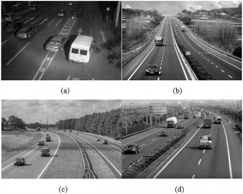
Figure 1. The original images: Test Image 1 (a), Test Image 2 (b), Test Image 3 (c), and Test Image 4 (d)
In the first test, the PSNR and MSE results obtained by the proposed method and the four classical methods (named Default, Global, VisuShrink, and NormalShrink, respectively) were compared. The tests were performed using four test images as shown in Figure 1. Each image had a size of 480×357 pixels, the horizontal and vertical resolution was 96 dpi, and the bit depth was 24. White noises with variations of 20, 30, 40 and 50 were added in the images. The results are given in Tables 2-5.
Table 2. Performance of the denoising methods of test image 1
|
|
σ=20 |
σ=30 |
σ=40 |
σ=50 |
||||
|
PSNR |
MSE |
PSNR |
MSE |
PSNR |
MSE |
PSNR |
MSE |
|
|
Default |
26.7089 |
138.7371 |
25.6244 |
178.0910 |
24.5950 |
225.7278 |
23.5936 |
284.2660 |
|
Global |
27.4071 |
118.1336 |
25.9249 |
166.1834 |
24.7125 |
219.6997 |
23.6119 |
283.0675 |
|
VisuShrink |
26.9899 |
130.0435 |
25.1662 |
197.9059 |
23.5208 |
289.0666 |
21.9318 |
416.7775 |
|
NormalShrink |
24.3661 |
237.9401 |
22.3466 |
378.8075 |
20.8292 |
537.2256 |
19.6111 |
711.1627 |
|
Proposed |
29.4964 |
73.0196 |
27.2145 |
123.4909 |
25.3248 |
190.8091 |
23.7741 |
272.6907 |
Table 3. Performance of the denoising methods of test image 2
|
|
σ=20 |
σ=30 |
σ=40 |
σ=50 |
||||
|
PSNR |
MSE |
PSNR |
MSE |
PSNR |
MSE |
PSNR |
MSE |
|
|
Default |
22.3611 |
377.5430 |
21.6585 |
443.8392 |
21.1543 |
498.4874 |
20.6470 |
560.2461 |
|
Global |
23.7380 |
274.9663 |
22.3634 |
377.3468 |
21.4703 |
463.4987 |
20.7769 |
543.7342 |
|
VisuShrink |
23.5279 |
288.5945 |
22.1107 |
399.9587 |
20.9619 |
521.0651 |
19.8194 |
677.8555 |
|
NormalShrink |
21.2498 |
487.6367 |
19.4918 |
730.9712 |
18.1446 |
996.8226 |
17.0462 |
1283.7 |
|
Proposed |
25.2100 |
195.9225 |
24.0410 |
256.4368 |
22.8648 |
336.1987 |
21.9228 |
417.6383 |
Table 4. Performance of the denoising methods of test image 3
|
|
σ=20 |
σ=30 |
σ=40 |
σ=50 |
||||
|
PSNR |
MSE |
PSNR |
MSE |
PSNR |
MSE |
PSNR |
MSE |
|
|
Default |
26.3191 |
151.7644 |
25.3897 |
187.9804 |
24.4911 |
231.1900 |
23.6029 |
283.6518 |
|
Global |
26.8908 |
133.0455 |
25.5634 |
180.6076 |
24.5359 |
228.8173 |
23.6234 |
282.3221 |
|
VisuShrink |
26.7652 |
136.9487 |
25.4722 |
184.4412 |
24.2164 |
246.2874 |
22.8114 |
340.3652 |
|
NormalShrink |
22.7158 |
347.9391 |
20.1216 |
632.2898 |
18.0501 |
1018.8 |
16.3904 |
1492.9 |
|
Proposed |
28.2714 |
96.8151 |
26.5885 |
142.6348 |
25.0894 |
201.4389 |
23.8805 |
266.0938 |
Table 5. Performance of the denoising methods of test image 4
|
|
σ=20 |
σ=30 |
σ=40 |
σ=50 |
||||
|
PSNR |
MSE |
PSNR |
MSE |
PSNR |
MSE |
PSNR |
MSE |
|
|
Default |
25.0348 |
203.9861 |
24.1379 |
250.7809 |
23.3943 |
297.6149 |
22.6556 |
352.7934 |
|
Global |
26.0216 |
162.5247 |
24.5782 |
226.5980 |
23.5312 |
288.3765 |
22.7067 |
348.6705 |
|
VisuShrink |
25.6977 |
175.1105 |
24.3006 |
241.5551 |
23.2572 |
307.1541 |
22.2822 |
384.4661 |
|
NormalShrink |
23.2568 |
307.1829 |
21.2546 |
487.1041 |
19.5947 |
713.8501 |
18.1831 |
988.0361 |
|
Proposed |
27.2681 |
121.9736 |
25.6948 |
175.2277 |
24.3248 |
240.2150 |
23.1729 |
313.1809 |
From the data in the Tables we can know that, for a same image, the results obtained by the proposed method were better than those of the other methods. For example, when white noise with a variance of 20 was added to test image 1, the PSNR result obtained by the proposed method was 29.4964 dB, which was increased by 2.7875 dB, 2.0893 dB, 2.5065 dB and 5.1303 dB respectively compared with the results obtained by Default, Global, VisuShrink and NormalShrink algorithms. In addition, the MSE result obtained by the proposed method was 73.0196, which was decreased by 65.7175, 45.1140, 57.0239 and 164.9205 respectively compared with the other four methods.
It was also found that the proposed method also outperformed the other four methods in different images. For instance, when white noise with a variance of 50 was added, compared with the other four methods, the PSNR result obtained by the proposed method increased by 0.5628 dB, 0.5079 dB, 1.4764 dB and 4.3391 dB, respectively.
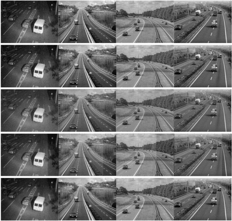
In the second test, noises with different intensities (σ=15, 20, 25, 30) were added to the four test images, which were subject to denoising tests, and the test results are shown in Figure 2. The images in the first row are results obtained by the Default method; the images in the second row are results obtained by the Globa method; the images in the third row are results obtained by the VisuShrink method; the images in the fourth row are results obtained by the NormalShrink method; and the images in the fifth row are results obtained by the proposed method. The results showed that the images in the first four rows are relatively blurred, the edges of feature objects such as traffic signs and vehicles are not prominent, and there’s obvious ringing artifacts. The proposed method outperformed the other four methods in the visual effect of the denoised images, and it can also retain the edge features of the images.
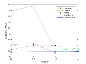
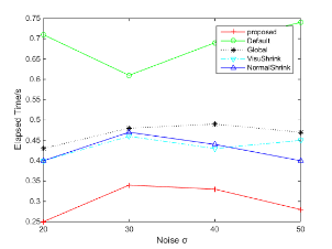
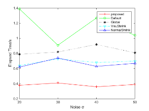
In the final test, the time complexity of the five algorithms was compared and the test results are shown in Figure 3. From Figure 3(a) we can see that, when the noise level σ was 20 and 30, the time required by the proposed algorithm was slightly longer than that of the Global method and the NormalShrink method, but the processing time of a single picture was only slightly more than 1s. When the noise level σ was greater than 40, the time required by the proposed algorithm was shorter than the other four methods, this might be related to the test images. From Figures 3(b), 3(c) and 3(d) we can know that, when the noise level σ was 20-50, the time required by the proposed algorithm was the shortest and it achieved good effects. Through comprehensive analysis we can see that, the proposed method is capable of real-time processing.
The reason for the good performance of the proposed algorithm is that, for wavelet coefficient of multi-layer decomposition, the more the layers, the smaller the noise energy becomes. Due to the adaptability of the threshold, the noise and useful information in each layer could be separated to the greatest extent. In addition, this paper selected the sym4 wavelet to decompose the images. The Sym4 wavelet has larger support width, and higher vanishing moment and regularity. Larger order of vanishing moment means the wavelet energy is concentrated, and higher regularity means that the two-dimensional images are smoother after reconstruction.
Figure 2. Visual effects of denoising results of four test images
Note: From left to right are test images 1, 2, 3, and 4 (σ=20). The first row: Default method; the second row: Global method; the third row: VisuShrink method; the fourth row: NormalShrink method; the final row: the proposed method.
(a)
(b)
(c)
(d)
Figure 3. Processing time required by five denoising methods for the four test images
Note: From left to right (a to d): results of test images 1, 2, 3 and 4, respectively.
This paper proposed an improved adaptive threshold denoising method suitable for WMSN image denoising. According to the different sub-band characteristics after the images were subject to wavelet decomposition, the scale parameter equation was defined to determine the adaptive optimal threshold suitable for each scale level; then combining with the proposed derivable threshold function and the optimal wavelet basis function selected by comparison, the images were subject to denoising processing. The proposed method was improved based the Donoho threshold denoising method, it could generate different thresholds suitable for each scale level and process different noise image signals. The test results showed that, the proposed method outperformed the classical methods in terms of visual effect and denoising performance, the method does not add time complexity and can be used for real-time processing.
This paper is supported by the Scientist Research Fund of Hunan Provincial Education Department under Grant No. 19B105, and the Scientist Research Project of Yiyang Technology Bureau under Grants No. YKZ(2016)51 & 2017YC01. The author would like to thank the anonymous reviewers for their insightful comments and suggestions, which have greatly improved this paper.
[1] Benrazek, A.E., Farou, B., Seridi, H., Kouahla, Z., Kurulay, M. (2019). Ascending hierarchical classification for camera clustering based on FoV overlaps for WMSN. IET Wireless Sensor Systems, 9(6): 382-388. http://dx.doi.org/10.1049/iet-wss.2019.0030
[2] Borawake-Satao, R., Prasad, R. (2019). Mobility aware multi-objective routing in wireless multimedia sensor network. Multimedia Tools and Applications, 78(23): 32659-32677. https://doi.org/10.1007/s11042-019-7619-z
[3] Medeiros, V.N., Silvestre, B., Borges, V.C.M. (2019). Multi-objective routing aware of mixed IoT traffic for low-cost wireless Backhauls. Journal of Internet Services and Applications, 10(1): 1-18. https://doi.org/10.1186/s13174-019-0108-9
[4] Baravdish, G., Svensson, O., Gulliksson, M., Zhang, Y. (2019). Damped second order flow applied to image denoising. IMA Journal of Applied Mathematics (Institute of Mathematics and Its Applications), 84(6): 1082-1111. https://doi.org/10.1093/imamat/hxz027
[5] Zou, Q., Poddar, S., Jacob, M. (2019). Sampling of planar curves: Theory and fast algorithms. IEEE Transactions on Signal Processing, 67(24): 6455-6467. https://doi.org/10.1109/TSP.2019.2954508
[6] Fletcher, A.K., Pandit, P., Rangan, S., Sarkar, S., Schniter, P. (2019). Plug in estimation in high dimensional linear inverse problems a rigorous analysis. Journal of Statistical Mechanics: Theory and Experiment, 2019(12). https://doi.org/1-10.10.1088/1742-5468/ab321a
[7] Gilda, S., Slepian, Z. (2019). Automatic Kalman-filter-based wavelet shrinkage denoising of 1D stellar spectra. Monthly Notices of the Royal Astronomical Society, 490(4): 5249-5269. https://doi.org/10.1093/mnras/stz2577
[8] Charmouti, B., Junoh, A.K., Mashor, M.Y., Ghazali, N., Wahab, M.A., Wan Muhamad, W.Z.A., Yahya, Z., Beroual, A. (2019). An overview of the fundamental approaches that yield several image denoising techniques. Telkomnika (Telecommunication Computing Electronics and Control), 17(6): 2959-2967. https://doi.org/10.12928/TELKOMNIKA.v17i6.11301
[9] Bal, A., Banerjee, M., Sharma, P., Maitra, M. (2019). An efficient wavelet and curvelet-based PET image denoising technique. Medical and Biological Engineering and Computing, 57(12): 2567-2598. https://doi.org/10.1007/s11517-019-02014-w
[10] Binbin, Y. (2019). An improved infrared image processing method based on adaptive threshold denoising. Eurasip Journal on Image and Video Processing, 2019(1): 1-12. https://doi.org/10.1186/s13640-018-0401-8
[11] Al-Naji, A., Tao, Y., Smith, I., Chahl, J. (2019). A pilot study for estimating the cardiopulmonary signals of diverse exotic animals using a digital camera. Sensors (Switzerland), 19(24): 1-14. https://doi.org/10.3390/s19245445
[12] Gilda, S., Slepian, Z. (2019). Automatic Kalman-filter-based wavelet shrinkage denoising of 1D stellar spectra. Monthly Notices of the Royal Astronomical Society, 490(4): 5249-5269. https://doi.org/10.1093/mnras/stz2577
[13] Chinna Rao, B., Madhavilatha, M. (2019). Fuzzy based adaptive thresholding or image denoising in complex wavelet domain. International Journal of Scientific and Technology Research, 8(11): 503-507.
[14] Rodrigues, C., Peixoto, Z.M.A., Ferreira, F.M.F. (2019). Ultrasound image denoising using wavelet thresholding methods in association with the bilateral filter. IEEE Latin America Transactions, 17(11): 1800-1807. https://doi.org/10.1109/TLA.2019.8986417
[15] da Silva Amorim, L., Ferreira, F.M.F., Guimarães, J.R., Peixoto, Z.M.A. (2019). Automatic segmentation of blood vessels in retinal images using 2D Gabor wavelet and sub-image thresholding resulting from image partition. Research on Biomedical Engineering, 35(3-4): 241-249. https://doi.org/10.1007/s42600-019-00028-9
[16] Nandal, S., Kumar, S. (2018). Image denoising using fractional quaternion wavelet transform. Advances in Intelligent Systems and Computing, 704: 301-313. https://doi.org/10.1007/978-981-10-7898-9_25
[17] Özmen, G., Özşen, S. (2018). A new denoising method for fMRI based on weighted three-dimensional wavelet transform. Neural Computing and Applications, 29(8): 263-276. https://doi.org/10.1007/s00521-017-2995-7
[18] Naragund, M.N., Jagadale, B.N., Priya, B.S., Panchaxri, Hegde, V. (2019). Improved image denoising with the integrated model of Gaussian filter and neighshrink SURE. International Journal of Engineering and Advanced Technology, 8(6): 3010-3015. https://doi.org/10.35940/ijeat.F9020.088619
[19] Koranga, P., Singh, G., Verma, D., Chaube, S., Kumar, A., Pant, S. (2018). Image denoising based on wavelet transform using Visu thresholding technique. International Journal of Mathematical, Engineering and Management Sciences, 3(4): 444-449.
[20] Verma, R., Pandey, R. (2018). Region characteristics-based fusion of spatial and transform domain image denoising methods. Turkish Journal of Electrical Engineering and Computer Sciences, 26(5): 2178-2193. https://doi.org/10.3906/elk-1802-52
[21] Stankiewicz, A., Marciniak, T., Dabrowski, A., Stopa, M., Rakowicz, P., Marciniak, E. (2017). Denoising methods for improving automatic segmentation in OCT images of human eye. Bulletin of the Polish Academy of Sciences: Technical Sciences, 65(1): 71-78. https://doi.org/10.1515/bpasts-2017-0009
[22] Akkar, H.A.R., Hadi, W.A.H., Al-Dosari, I.H.M. (2019). Implementation of sawtooth wavelet thresholding for noise cancellation in one dimensional signal. International Journal of Nanoelectronics and Materials, 12(1): 67-74.
[23] Mafi, M., Tabarestani, S., Cabrerizo, M., Barreto, A., Adjouadi, M. (2018). Denoising of ultrasound images affected by combined speckle and Gaussian noise. IET Image Processing, 12(12): 2346-2351. https://doi.org/10.1049/iet-ipr.2018.5292
[24] Venuji Renuka, S., Reddy Edla, D. (2019). Adaptive shrinkage on dual-tree complex wavelet transform for denoising real-time MR images. Biocybernetics and Biomedical Engineering, 39(1): 133-147. https://doi.org/10.1016/j.bbe.2018.11.003
[25] Khmag, A., Ramli, A.R., Kamarudin, N. (2019). Clustering-based natural image denoising using dictionary learning approach in wavelet domain. Soft Computing, 23(17): 8013-8027. https://doi.org/10.1007/s00500-018-3438-9
[26] Diwakar, M., Kumar, M. (2018). CT image denoising using NLM and correlation-based wavelet packet thresholding. IET Image Processing, 12(5): 708-715. https://doi.org/10.1049/iet-ipr.2017.0639
[27] Fahmy, M.F., Fahmy, O.M. (2018). Efficient bivariate image denoising technique using new orthogonal CWT filter design. IET Image Processing, 12(8): 1354-1360. https://doi.org/10.1049/iet-ipr.2017.1117
[28] Naragund, M.N., Jagadale, B.N., Priya, B.S., Panchaxri, Hegde, V. (2019). An efficient image denoising method based on bilateral filter model and neighshrink SURE. International Journal of Recent Technology and Engineering, 8(3): 8470-8475. https://doi.org/10.35940/ijrte.C6629.098319
[29] Bascoy, P.G., Quesada-Barriuso, P., Heras, D.B., Argüello, F. (2019). Wavelet-based multicomponent denoising profile for the classification of hyperspectral images. IEEE Journal of Selected Topics in Applied Earth Observations and Remote Sensing, 12(2): 722-733. https://doi.org/10.1109/JSTARS.2019.2892990
[30] Agarwal, S., Singh, O.P., Nagaria, D. (2017). Analysis and comparison of wavelet transforms for denoising MRI image. Biomedical and Pharmacology Journal, 10(2): 831-836. https://doi.org/10.13005/bpj/1174