Akram Isvand Rahmani* | Moosa Katouli
OPEN ACCESS
Today’s, of the major cancers for both females and male is lung cancer. This type of cancer is the most common cause of mortality that accounts for up to 20% of all cancers. The incidence of this cancer has noticeably increased since the beginning of the 19th century. The current study aims to investigate and present a novel method to diagnose lung cancer using Optimization Algorithm (GOA) algorithm and KNN classification. The study method includes three steps. In the first step, pre-processing of lung cancer cell data is used to remove irrelevant and duplicate features. In the second step, the Grasshopper Optimization Algorithm (GOA) method is used to select the high-dimensional feature. In the third step, the selected features are classified into three categories, namely low, medium and high using the KNN nearest neighbor classifier. To evaluate the proposed method, the UCI dataset is used. The results indicate that this method has superior performance with the accuracy of 98.65, specificity of 96.7, and sensitivity of 94.10, demonstrating the superiority of this method over others. The results show that diagnosis of lung cancer using data mining techniques provides the physician with the most detailed and accurate information in the shortest possible time.
mortality, high-dimensional feature, categories, UCI dataset, data mining
Lung cancer is the uncontrolled growth of cells beginning with one or more cells. Unusual cells do not grow in healthy tissues, and they divide rapidly and form tumors. Primary lung cancer originates in the lungs, while secondary lung cancer begins elsewhere in the body, spreading from one body point to another and reaching the lungs. As investigated in many studies, detection of cancer in the patient's body through early symptoms is necessary [1].
In 2015, in a comprehensive investigation of 589430 mortalities from cancer has been announced that the most common causes of cancer mortalities were lung cancer both among women and men so that more than 1.4%, 27% of all mortalities are caused by it [2].
Regarding that lung cancer is one of the most dangerous cancers, applying sufficient diagnostic methods in the early stages of its development can be very critical to treat the patient [1]. This early diagnosis can help physicians to treat patients as well as to greatly decrease the mortality of patients. It also increased the 5-year survival rate of patients with this cancer from 14% to 49%. Distinguishing the pulmonary nodules is particularly important in early diagnosis of lung cancer, because about 20% of cases of pulmonary nodules represent lung cancer [2]. As the lung nodules are small and dense masses in the human lung, they sometimes are difficult to distinguish blood vessels that form circular spots. It should be noted that eye diagnosis can be error prone, based on which the radiologist may not diagnose both the nodule and cancer [3]. The features of lung cancer are extracted to predict the stage of cancer based on the specific features used in the system. In this way, the feature selection is employed to identify the predicted datasets of cancer cells and reduce the number of cancer cells provided by the calculation method. Meanwhile, the better performance can be achieved through removing some features. In this paper, the dimension reduction method and its effect on the diagnosis of lung disease have been investigated. As such, this paper aims to improve the classification accuracy, increase the rate of correct diagnosis, and reduce the rate of incorrect to predict lung cancer. To achieve this aim, a novel and practical hybrid approach of Grasshopper Optimization Algorithm (GOA) is developed to reduce feature dimensions as well as the k-Nearest Neighbor (KNN) algorithm. It is worthwhile to mention that up to now, no such algorithm has been implemented for the diagnosis of lung cancer.
This paper is organized as follows: Section 2 describes an overview of the known methods of dimensionality reduction. Section 3 investigates the effect of grasshopper optimization algorithm on dimensionality reduction in lung cancer diagnosis systems. Section 4 evaluates the methods investigated, along with the table and comparisons of the results and their analysis. Finally, Section 5 presents the conclusions.
Yung et al. [4] have discussed several data mining methods used to diagnose cancer. Establishment (presentation) of lung cancer pathology based on the pathology report to describe the size or the expansion of the primary tumor and whether the cancer has a growth or not (it has metamorphosis). Being aware of the establishment of lung cancer pathology, because it can be used to predict patient status, can also help physicians plan appropriate treatment [5]. Tissue specimens from the patient's lung were required to complete the pathology report to diagnose the pathology of the lung cancer. Although in this process, biopsy surgery is necessary, it may put the patient's health at risk [6]. As a result, this paper focused on obtaining clinical information that can be provided without surgery to place the pathology report. In this regard, data mining techniques have been utilized to explore the relationship between clinical information and pathology reports to support the establishment of a diagnosis of lung cancer pathology. This method is time-consuming and complex due to selection of features.
Ahmad et al. [7] stated a detailed research on lung cancer diagnosis by gathering 400 data on cancerous and non-cancerous patients from different diagnostic centers, preprocessing it and using the k-means clustering algorithm to identify relevant and non-relevant data. Moreover, some subsequent significant duplicate patterns were also designed using the Aprioritid and Decision Tree (DT) algorithm. Ultimately, with the use of predictive tools for the meaningful patterns, lung cancer diagnosis systems were developed. This lung cancer risk prediction system must be proven in the diagnosis of one's readiness for lung cancer. .This method cannot be considered reliable, since is no specific procedure for computing preliminary cluster centers for each k-means cluster, and the final answer depends on selection of preliminary clusters.
Another study [8] proposed a Computer-Aided Diagnostic (CAD) method in Computer Tomography (CT) images for a neural network based on cancer diagnosis. In this paper, whole lungs are separated from CT images, in which some features are separated from the split image. The, some measurable parameters such as mean, standard deviation, fat, short-sighted, fifth and sixth focal moment are estimated for cancer classification. The classification process is performed using forward and backward propagation neural networks for better classification. Accurate estimation of parameters is the advantage of this method.
Senthil and Ayshwarya [1] describes a computerized classification method to predict lung cancer based on an evolutionary system with a hybrid of architectural evolution through learning weights by utilizing Neural Network (NN) and Particle Swarm Optimization (PSO) have been implemented. It employed a variety of combinations of methods and enhanced its evolutionary algorithm using PSO feature selection along with a local search of the neural network to predict lung cancer as a non-cancerous disease.
The study [9] evaluated a new feature selection technique using hybrid genetic optimization and particle optimization and classification of lung CT images using MLP-NN. It is attached to the lung CT images, which are attached as inputs. Afterwards, the conducted image filters to remove noise are attached and then the preprocessed images are provided as input for feature extraction. Besides, the features are extracted using the MAD technique. The extracted features are chosen using GAPSO algorithm. Furthermore, the properties are finally classified using MLP-NN. The resulting image is achieved using GAPSOMLPNN. The test results reveal high geometrical accuracy, high bit rate classification, and low bit error rate in the different test data. This method is remarkable enough to diagnose lung disease. The disadvantage of meta-heuristic methods such as GAPSO and pso is the local optimality that considers only the current solution, which cannot be compared to the previous solutions.
To solve the local optimality problem in the proposed method, the GOA algorithm is used to reduce the dimension. Therefore, the present study aims to enhance the classification accuracy, increase the rate of correct prediction, and reduce the rate of incorrect perdition in lung systems. To accomplish this aim, a novel grasshopper Optimization Algorithm (GOA) is developed to reduce both feature dimensions and k-Nearest Neighbor (KNN). It is worthwhile to mention that no such algorithm has been developed so far to predict lung cancer. In this regard, we will describe the algorithm in more detail in the next section [10].
3.1 Pre-processing
Data pre-processing is performed to check for duplicate data, noise removal, and unspecified values. In the proposed method, the feature vector obtained in the previous step is pre-processed to check for any noise (missing value, duplicate and error values) in the dataset [11].
3.2 Grasshopper optimization algorithm
Here, it should be mentioned that optimization in the old ways, like optimization with mathematical methods, mainly works on the information derived from the objective function derivative to find the optimum solution. Although such techniques are still used by various researchers, these methods contain some disadvantages. Mathematical optimization methods suffer from being stuck to local optimum points, that is, the algorithm assumes a local optimum solution as a global optimum solution, and thus will not be able to find the global optimum. In contrast, the mathematical methods are also often not applicable to solve such problems where their derivatives are not known or not derivable [12]. Now, the grasshopper optimization algorithm that, in essence, mimics grasshopper swarm behavior, which is affected by three components that are mathematically represented by Eq. (1):
${{\text{X}}_{\text{i}}}\text{=}{{\text{S}}_{\text{i}}}\text{+}{{\text{G}}_{\text{i}}}\text{+}{{\text{A}}_{\text{i}}}$ (1)
where, in the Eq. (1), the Xj denotes the position of the grasshopper i, the Si of social interaction, the Gi gravitational force on the i grasshopper, the Ai horizontal force at the direction of movement i on the grasshopper. Moreover, the random behavior of Eq. (1) can be re-written as $\mathrm{X}_{\mathrm{i}}=\mathrm{r}_{1} \mathrm{S}_{\mathrm{i}}+\mathrm{r}_{2} \mathrm{G}_{\mathrm{i}}+\mathrm{r}_{3} \mathrm{A}_{\mathrm{i}}$ in which $r_{1}, r_{2}$ and $r_{3}$ can be a random digit between 0 and 1 [12].
The social interaction is the main search mechanism of the GOA algorithm that is computed as Eq. (2):
$\mathrm{X}_{\mathrm{i}}=\mathrm{S}_{\mathrm{i}}+\mathrm{G}_{\mathrm{i}}+\mathrm{A}_{\mathrm{i}} \mathrm{S}_{\mathrm{i}}=\sum_{\mathrm{j}=1, \mathrm{j} \neq \mathrm{i}}^{\mathrm{N}} \mathrm{s}\left(\mathrm{d}_{\mathrm{ij}}\right) \hat{\mathrm{d}}_{\mathrm{ij}}$ (2)
where, $d_{i j}$ is the distance between ith and jth grasshopper and denoted as ${{\text{d}}_{\text{ij}}}\text{=}\left| {{\text{x}}_{\text{j}}}\text{-}{{\text{x}}_{\text{i}}} \right|$, Is also defined, $\hat{\mathrm{d}}_{\mathrm{ij}}$ is a singular vector of the ith grasshopper to the ith grasshopper that is $\hat{\mathrm{d}}_{\mathrm{ij}}=\frac{\mathrm{X}_{\mathrm{j}}-\mathrm{X}_{\mathrm{i}}}{\mathrm{d}_{\mathrm{ij}}}$ calculated and, finally, s is a function of the power of social interaction expressed in Eq. (3) [12].
$\mathrm{S}(\mathrm{r})=\mathrm{fe}^{\frac{-\mathrm{r}}{1}}-\mathrm{e}^{-\mathrm{r}}$ (3)
where, f is the gravitational intensity and l represents the scale of the gravitational length of social interaction. However, the component G, which represents the gravitational force, is calculated in Eq. (4).
$\mathrm{G}_{\mathrm{i}}=-\mathrm{g} \hat{\mathrm{e}}_{\mathrm{g}}$ (4)
In the above relation, g is the gravitational constant, $\widehat{\boldsymbol{e}_{\mathrm{g}}}$ A singlural vector is toward the center of the Earth. Finally, component A, which represents the horizontal force of the wind, is calculated in Eq. (1) to (5):
$\mathrm{A}_{\mathrm{i}}=\mathrm{u} \widehat{\mathrm{e}_{\mathrm{w}}}$ (5)
Here, u constant drift, $\widehat{e_{w}}$; is a singular vector in the wind direction. As it is known, as newborn grasshoppers have no whales, so their movement is strongly associated with wind. Thus, by substituting S, G and A in Eq. (1), the Relation can be rewritten as Eq. (6):
$\mathrm{X}_{\mathrm{i}}=\sum_{\mathrm{j}=1, \mathrm{j} \neq \mathrm{i}}^{\mathrm{N}} \mathrm{s}\left|\mathrm{x}_{\mathrm{i}}-\mathrm{x}_{\mathrm{j}}\right| \frac{\mathrm{x}_{\mathrm{j}}-\mathrm{x}_{\mathrm{i}}}{\mathrm{d}_{\mathrm{ij}}}-\mathrm{g} \widehat{\mathrm{e}_{\mathrm{g}}}+\mathrm{u} \widehat{\mathrm{e}_{\mathrm{w}}}$ (6)
where, $\mathrm{s}(\mathrm{r})=\mathrm{fe}^{\frac{-\mathrm{T}}{1}}-\mathrm{e}^{-\mathrm{r}}$ and N are the number of grasshoppers. As the newborn grasshoppers are on the ground, their position should not be below the threshold level. However, Saremi et al. [12] refined the optimization algorithm, while the grasshoppers interact, was described as in Eq. (7):
$\mathrm{X}_{\mathrm{i}}^{\mathrm{d}}=\mathrm{c}\left(\sum_{\mathrm{j}=1, \mathrm{j} \neq \mathrm{i}}^{\mathrm{N}} \mathrm{c} \frac{\mathrm{ub}_{\mathrm{d}^{-}} \mathrm{lb}_{\mathrm{d}}}{2} \mathrm{s}\left(\left|\mathrm{x}_{\mathrm{j}}^{\mathrm{d}}-\mathrm{x}_{\mathrm{i}}^{\mathrm{d}}\right|\right) \frac{\mathrm{x}_{\mathrm{j}}-\mathrm{x}_{\mathrm{i}}}{\mathrm{d}_{\mathrm{ij}}}+\widehat{\mathrm{T}}_{\mathrm{d}}\right.$ (7)
where, $u b_{d}$ upper bound in the dimension d, $l b_{d}$ lower bound in the dimension d, is an c the best solution so far, and $\hat{\mathrm{T}}_{\mathrm{d}}$ increasing coefficient to reduce the comfort zone, the repulsion zone and the gravitational force zone.
Therefore, $c \frac{u b_{d}-l b_{d}}{2}$ is an equation that is linearly the space that reduces the grasshoppers should explore and exploit.
The equation $\mathrm{s}\left(\left|\mathrm{x}_{\mathrm{j}}^{\mathrm{d}}-\mathrm{x}_{\mathrm{i}}^{\mathrm{d}}\right|\right)$ indicates whether a grasshopper should be removed from the target (or explored) or aim to be absorbed. To balance exploration and exploitation, the parameter c must be reduced in proportion to the number of iterations. This mechanism increases the number of interactions in operation. The coefficient c decreases the comfort zone according to the number of interactions and is calculated as Relation (8):
$\mathrm{c}=\mathrm{cmax}-1 \frac{\text { cmax-cmin }}{\mathrm{L}}$ (8)
where, "cmax" is the maximum value, "cmin" is the minimum value.
3.3 feature reduction by GOV-KNN
In general, the higher the dimensions or properties of the problem being explored, the more likely the records will be in the search space. The selection of a subset of features is one of these methods. Here, those properties whose information value is lower will be eliminated. For this reason, there are usually not many features that will be ignored in this way. Thus, a subset of feature selection operations cannot be considered as effective to solve such problems with a high number of features. In feature selection operations, it is also important to solve the problem of preserving the nature of features to reserve model interpretation capability. Note that the feature selection is a binary optimization problem, where its solutions are limited to binary values of {0, 1}. For this reason, a grasshopper optimization algorithm was developed to facilitate the high dimensional feature-based solution to the optimization algorithm [13]. Outlined by Goldberg et al. [14], the tournament selection is a simple tool but practical to implement the selection mechanism. This method is one of the best selection mechanisms in the evolutionary algorithms. In the contest selection, n solutions are randomly selected from the population. Afterwards, these solutions are compared against each other and then placed to specify the winner in the competition [15]. As these competitions involve generating a random number between 0 and 1, compared with a probability 1 of selection, which is the appropriate mechanism for adjusting the selection pressure (usually set to 0.5). If the random number is larger, a solution with the highest proportion will be chosen; otherwise the weak solution will be selected. This feature in the tournament selecting is an opportunity to make more choices that have a variety of decision-making.
Therefore, A solution is provided in one-dimensional vector, such that the length of the vector is based on the number of features of the original dataset. Each value in the vector is represented by 1 or 0. The value of 1 indicates that the corresponding feature is selected; otherwise, the value is set to 0 and means no feature is selected. Feature selection can be considered as a multi-objective optimization problem where two opposing objectives are achieved; the minimum number of features selected and the higher classification accuracy [13].
Note that as the lower the number of features, the higher the classification accuracy and the better the solution. Each solution will be calculated based on the fitness function, which depends on the accuracy and number of features selected and the KNN classifier. Now, to balance the number of features selected in each solution (minimum) as well as classification accuracy (maximum), the fitness function in Eq. (9) is employed to search for factors in the grasshopper algorithm:
fitness$=\alpha \gamma_{R}(D)+\beta \frac{|R|}{|N|}$ (9)
In Eq. (9), $\gamma_{R}(\mathrm{D})$ the classification error rate of the given classifier (here KNN classifier) is used, $|R|$ Powerful subsets of selected features and $|N|$. The sum of the properties selected is in the dataset. Two parameters α and β are related to the importance of classification quality and subset length, which are defined as $\alpha \in[0,1]$ and $\beta=(1-\alpha)$ [16].
As mentioned in the Grasshopper Algorithm, the utilization depends on calculating the distance between the search factor and the most known grasshopper to date. Therefore, one can improve the results by using the local search algorithm around the best-known solution such as Eq. (8). Furthermore, Based on Eq. (7), as the exploration in the grasshopper algorithm is dependent on changing the position of each search agent based on a random solution, it can be improved by using different selection mechanisms such as the tournament selection [16].
This means that the tournament selection method provides more opportunity for poorly chosen solutions during the search process based on the selective pressure that improves the ability of the grasshopper algorithm diversity [16].
At the end, what can be summarized in the proposed method based on data from the lung disease classification system is carried out after preprocessing to normalize the data. In addition, the grasshopper algorithm is employed to choose the best features to reduce the feature. Then, using the KNN classifier algorithm, the lung disease is classified into three modes of low, medium and high data. It should be noted that such a procedure has not yet been performed on lung diagnosis.
This Section includes the results of the implementation and testing of dimensionality reduction techniques in the lung classification system using the Grasshopper Properties Reduction Algorithm and the KNN. The Section 4-1 of the dataset is used, along with information about it. The Section 4-2 presents the evaluation criteria and the Section 4-3 selects the classification parameters. Finally, the results of the experiments and comparisons, as well as the conclusions in Section 4-4, are presented.
4.1 Datasets
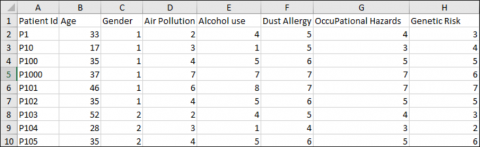
To evaluate the proposed method, the UCI dataset [17] was used. In this dataset, the characteristics of symptoms of lung disease are used. These include age, gender, air pollution, alcohol use, dust Allergy, occupation hazard, chronic lung disease, balanced diet, obesity, smoking, passive smoking, chest pain, blood cough, fatigue, weight loss Diarrhea, wheezing, difficulty swallowing, fingernail cramping, frequent colds, dry cough and snoring have been considered to predict lung cancer. An example of this dataset is shown in Figure 1.
Figure 1. Part of the dataset
The total features of this dataset contain 24 features that use 23 numerical features of the dataset to analyze the performance of the proposed method. Three categories of low, medium and high tags were undertaken to classify this dataset.
4.2 The evaluation criteria
The KNN evaluates the reduced data derived from the methods outlined in the previous Section. In this Section, the reduced data are classified as training and test data for classification of the data. 10-fold cross validation is used for dividing the data. The evaluation criteria considered for test data include accuracy, specificity and sensitivity.
In classifying and identifying the bid, it leads to 4 True Positive, True Negative, False Positive and False Negative.
To obtain the values listed above, the above values are described as follows:
4.2.1 Accuracy
Accuracy refers to a measure of how well a model's predictions fit, which is consistent with the modeled reality [18]. The criterion of accuracy means the proximity of the measured values to the real value obtained from the Relation (10):
Acurency $=\frac{T_{p}+T_{N}}{N}$ (10)
4.2.2 Specificity
Specificity means a proportion of negative cases that the experiment correctly marks as negative. The Specificity Criterion refers to the same concept for healthy people (or the negative category); that is, how many truly healthy people have been correctly identified from all healthy people
Specificity $=\frac{\text { mumber of true negatives }}{\text { mumber of true negatives + number of false negatives }}$ (11)
4.2.3 Sensitivity
Sensitivity means a proportion of positive cases that the test correctly marks as positive. In fact, we have identified a criterion that shows how many actual (positive) patients are in relation to the complete patient population. That is, the proportion of correctly identified patients to the sum of all patients (correctly identified patients + wrongly prediction healthy patient). The target is to have a high sensitivity of the model, meaning to identify more patients. In a view of mathematically speaking, sensitivity is the result of dividing the real positive into the sum of the real positive and the negative [12].
sensitivity $=\frac{\text { number of true positives }}{\text { mumber of true positives + mumber of false negatives }}$ (12)
In these experiments, the evaluation criteria were evaluated for the entire dataset with 23 features, without any dimensionality reduction.
4.3 Selecting the classification parameters
The implemented experiments on the methods have been performed by MATLAB 2016 software on Corei5 processor and 4 GB main memory. In the present study, the accuracy of the classification of the data reduced by the k-Nearest Neighbor Classification (KNN) data with different values of k (i.e., 3, 5 and 7) has been tested and evaluated, with this class of data The reduced data are trained, then evaluated with the test data of these classifiers.
4.4 Evaluation and comparison
In this Section, the results of the experiments are reported. At first, the results of the experiments without dimension reduction in the desired dataset, with 23 properties, are listed in Table (1). Then, the results of KNN classification with different number of features are analyzed and provided by table and graph drawing. In addition, the best results are obtained with some popular methods presented in the field of genetic cancer prediction [20], particle swarm optimization [1] and Whale Optimization Algorithm [13] and Ant Lion Optimizer [21] are compared. Table (1) shows the accuracy, specificity and sensitivity performance of the proposed method in the case of k=3, 5, 7.
Table 1. The results of the KNN classifier with different values
|
accuracy |
specificity |
Sensitivity |
KNN classifier |
|
98.65 |
96.7 |
94.1 |
K = 3 |
|
99.8 |
97.2 |
95.6 |
K = 5 |
|
97.3 |
95.21 |
93.11 |
K = 7 |
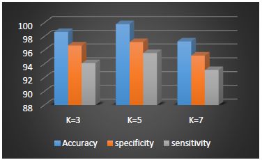
As illustrated in Figure 2, k = 5 performs better in all cases. Therefore, this case has been investigated for comparison with other methods. Table 2 shows the performance, accuracy, specificity, and sensitivity of the proposed method to other methods.
Comparative performance can be shown in Figure 2, given the superiority of the proposed method over other feature reduction methods.
Figure 2. The results of the KNN classifier with values of k
Table 2. Comparison of different methods
|
sensitivity |
specificity |
Accuracy |
Methods |
|
93.5 |
91.7 |
95.4 |
Genetic [22] |
|
92 |
94.8 |
97.8 |
Particle swam optimization [1] |
|
94.3 |
89.6 |
93.2 |
ant optimization [21] |
|
90.3 |
95.2 |
98.1 |
Whale Optimization Algorithm [13] |
|
94.10 |
96.7 |
98.65 |
KNN classifier with the value K = 3 proposed method with GOA |
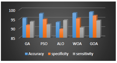
Figure 3. Results of different methods
As depicted in Figure 3, the performance of the proposed method is at the forefront given the very close proximity to Particle Swarm Optimization (PSO) and Whale Optimization (WOA). At the meantime, other Particle Swarm Optimization (PSO) and Whale Optimization (WOA) algorithms fall into the second and third ranks, respectively. Genetic algorithm also performs better than ant lion optimization, ranking fourth and fifth respectively. It should be noted that the number of iterations for the GOA algorithm is 100. It should be noted that all the results were obtained 200 times with cMAX = 2.079 and cMIN = 0.00004 parameters.
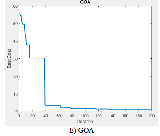
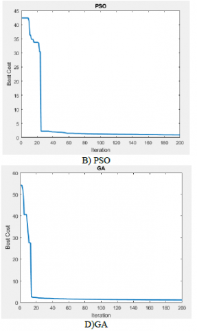
In short, it can be said that the proposed method performs better than the other methods. The PSO method comes in second, as it considers only the local and global position of each particle while does not consider the optimum solution over other solutions. The Genetic methods, however, are ranked third in each population due to the randomness of the initial population and the different solutions to each of the crossover and mutation operations, making each replication different in magnitude. Whale and Ant lion optimization methods fall into the fourth and fifth ranks, respectively. We now discuss the convergence of the proposed method with respect to other methods (Figure 4).
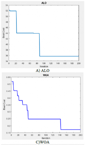
Figure 4. The convergence diagram of different feature reduction methods
As can be seen in Figure 4, in the GOA method, when the replication reaches close to 140, the objective function converges and reaches its minimum. The GOA method performs very closely with the WOA, but is still less than its objective function. The PSO method is also closely related to two mentioned methods, which fall into the third category in terms of decreasing the objective function value. The value of the genetic and ALO objective function in this experiment is in the following categories.
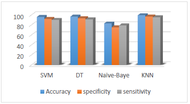
After investigating the convergence of the feature reduction, the following Section assesses the performance of the different classes according to the proposed method. The classes of comparable categories are SVM, KNN, DT and table Naïve-Bayes (see Table 3).
Table 3. Comparing the different classifiers
|
sensitivity |
specificity |
Accuracy |
Classifier |
|
90.46 |
92.47 |
96.38 |
SVM |
|
91.56 |
93.98 |
97.14 |
DT |
|
79.43 |
75.66 |
83.23 |
Naïve-Bayes |
|
95.6 |
97.2 |
99.8 |
KNN |
Figure 5. Comparing the performance of different classifiers
Regarding the performance of KNN and decision tree classifiers in Figure 5, it can be considered that with regard to the speed of these two classifiers that have for data training and testing, they can be utilized for datasets. Besides, larger ones will also be used. These classifiers have been used with the 10-K-fold validation model.
In this study, we propose a classification method for grasshopper optimization based on grasshopper optimization. The proposed method is mathematically modeled and imitated the behavior of grasshoppers in nature to solve optimization problems. The k-Nearest Neighbor Classifier (KNN) and its results then evaluated the reduced data obtained from these methods. Then the proposed method was compared with other methods based on genetic algorithm, particle swarm and ant lion optimization (Alo). The results show that the proposed method is capable of diagnosing diseases in three low, medium and high states, and its quantitative performance results are very close to the optimum Particle Swarm Optimization (PSO) and the KNN classification performs best among the classes. It has different clauses. It should be noted that the method of diagnosis of lung cancer by Grasshopper Optimization Algorithm (GOA) has not been investigated. In the future, we will also use this method to detect breast cancer.
[1] Senthil, S., Ayshwarya, B. (2018). Lung cancer prediction using feed forward back propagation neural networks with optimal features. Journal of Applied Engineering Research, 13(1): 318-325.
[2] Farhood, B., Geraily, G., Alizadeh, A. (2018). Incidence and mortality of various cancers in Iran and compare to other countries. Iranian Journal of Public Health, 47(3): 309-316.
[3] Tiwari, A. (2016). Prediction of lung cancer using image processing techniques: A review. Advanced Computational Intelligence: An International Journal (ACII), 3: 1-9. https://doi.org/10.5121/acii.2016.3101
[4] Yang, H.F., Chen, Y.P. (2015). Data mining lung cancer pathologic staging diagnosis: Correlation between clinical and pathologic information. Expert Systems with Applications, 42(15-16): 6168-6176. https://doi.org/10.1016/j.eswa.2015.03.019
[5] Hussain, R.Q., Aziz, A. (2017). Detection of lung cancer in smokers and non-smokers by applying data mining techniques. Indian Journal of Science and Technology, 10(33): 1-5. https://doi.org/10.17485/ijst/2017/v10i33/114700
[6] Bharathi, H., Arulananth, T.S. (2017). A review of lung cancer prediction system using data mining techniques and self organizing map (SOM). Journal of Applied Engineering Research, 12(11): 2190-2195.
[7] Ahmad, K., Emran, A.A., Jesmin, T., Mukti, R.F., Rahman, M.Z., Ahmed, F. (2013). Early detection of lung cancer risk using data mining. Asian Pacific, 14(1): 595-598. https://doi.org/10.7314/apjcp.2013.14.1.595
[8] Kuruvilla, J., Gunavathi, K. (2014). Lung cancer classification using neural networks for CT images. Computer Methods and Programs in Biomedicine, 113(1): 202-209. https://doi.org/10.1016/j.cmpb.2013.10.011
[9] Kaur, T., Gupta, N. (2015). Classification of lung diseases using particle swarm optimization. Journal of Advanced Research in Electronics and Communication Engineering (IJARECE), 4(9): 2440-2446.
[10] Ibrahiim, H.T., Mazher, W.J., Ucan, O.N., Bayat, O. (2018). A grasshopper optimizer approach for feature selection and optimizing SVM parameters utilizing real biomedical data sets. Neural Computing and Applications, 31: 5965-5974. https://doi.org/10.1007/s00521-018-3414-4
[11] Shyamala, S., Pushparani, M. (2016). Pre-processing and segmentation techniques for lung cancer on CT images. International Journal of Current Research, 8: 31665-31668.
[12] Saremiab, S., Mirjalili, S., Lewisa, A. (2017). Grasshopper optimisation algorithm: Theory and application. Advances in Engineering Software, 105: 30-47. https://doi.org/10.1016/j.advengsoft.2017.01.004
[13] Mafarja, M., Mirjalili, S. (2017). Hybrid whale optimization algorithm with simulated annealing for feature selection. Neurocomputing, 260: 302-312. https://doi.org/10.1016/j.neucom.2017.04.053
[14] Goldberg, D., Korb, B., Deb, K. (1989). Messy genetic algorithms: Motivation, analysis, and first results. Complex Systems, 3(5): 493-530.
[15] Sanchita, G., Anindita, D. (2016). Evolutionary algorithm based techniques to handle big data. Techniques and Environments for Big Data Analysis. Studies in Big Data, 17: 113-158. https://doi.org/10.1007/978-3-319-27520-8_7
[16] Emary, E., Zawbaa, M., Hassanien, A.E. (2016). Binary ant lion approaches for feature selection. Jornal of Neurocomputing, 213: 54-65. https://doi.org/10.1016/j.neucom.2016.03.101
[17] Christopher, T., Jamera banu, J. (2016). Study of classification algorithm for lung cancer prediction. Journal of Innovative Science, Engineering & Technology, 3(2): 42-49.
[18] Krishnaiah, V., Narsimha, G., Subhash Chandra, N. (2013). Diagnosis of lung cancer prediction system using data mining classification techniques. International Journal of Computer Science and Information Technologies, 4: 39-45.
[19] Toyoda, Y., Nakayama, T., Suzuki, T. (2008). Sensitivity and specificity of lung cancer screening using chest low-dose computed tomography. British Journal of Cancer, 1602-1607.
[20] Bhuvaneswari, P., Therese, A.B. (2015). Detection of cancer in lung with K-NN classification using genetic algorithm. Procedia Materials Science, 10: 433-440. https://doi.org/10.1016/j.mspro.2015.06.077
[21] Senthil, S. (2019). Improving the performance of lung cancer detection at earlier stage and prediction of reoccurrence using the neural networks and ant lion optimizer. International Journal of Recent Technology and Engineering (IJRTE), 8(2): 6378-6391.
[22] Desale, K., Roshani, A. (2015). Genetic algorithm based feature selection approach for effective intrusion detection system. International Conference on Computer Communication and Informatics (ICCCI), India. https://doi.org/10.1109/ICCCI.2015.7218109